Matthew’s Blog - Neural Networks and Calculus

In a recent workshop the fundamentals of calculus as they relate to Neural Networks was introduced. The discussion was based around the simplest possible problem, a classification problem:

So the problem is to determine if a given point is above the line or not. It looks like an easy problem, but how do you actually mathematically do it?

Problem as Equation

Well the proposed network that would solve this is as follows:

If we want to express the classification problem as such a network then we can. The inputs to the network are x and y because the problem is two dimensional. Then we can also add in a bias term:

We can express this network as an equation quite easily:

\[ \begin{aligned} z &= \sum_{k=1}^{n} x_k \cdot w_k \\ z &= w_x \cdot x + w_y \cdot y + w_{bias} \end{aligned} \]

Then we can plug this into sigmoid, which is our activation function:

\[ σ = \frac{1}{1 + e^{-z}} \]

Which then leads to:

\[ \begin{aligned} a &= \frac{1}{1 + e^{-(w_x \cdot x + w_y \cdot y + w_{bias})}} \\ a &= \frac{1}{1 + e^{-w_x \cdot x - w_y \cdot y - w_{bias}}} \end{aligned} \]

I really need to fix the blog rendering.

Loss

The way that neural networks solve this is by defining a function which calculates a loss value. The loss value is a measure of the current quality of the network.

To know what a good value of the network is we should think about the classification problem again. We really have two classes to predict - above the line or below the line. The sigmoid function naturally scales any input to a value between zero and one. So we can choose zero for the points below the line and one for the points above the line.

If we can define a loss value for the network then can we determine what values can be used for the weights? A neural network wants a loss that is always positive, continuous and where a lower value is better than a higher one.

I am really dragging this out.

This means that for points above the line the best value is 1. That should have a loss of 0. Equally points below the line have a best value of 0. The distance to the best point is an ideal loss value.

We also want this loss to be continuous. If we take the absolute difference between \(a\) and the best value then it is not continuous at the best value. Instead we can take the square of the difference, as that is nice and smooth.

\[ \begin{aligned} loss_0 &= \left( \frac{1}{1 + e^{-w_x \cdot x - w_y \cdot y - w_{bias}}} \right)^2 \\ loss_1 &= \left( \frac{1}{1 + e^{-w_x \cdot x - w_y \cdot y - w_{bias}}} - 1 \right)^2 \end{aligned} \]

The loss across many data points is the mean sum of the individual losses. Since the individual loss is the square of the difference between the actual value and the desired value (i.e. the error), this leads to the name mean square error for this loss (often abbreviated to mse).

Solving for One Variable

So if I were to fix two of the three variables can I derive the other variable? I can if I define a few data points and then calculate the average loss.

Let’s start by defining what the values should be. A simple solution to this classification problem is:

\[ 0 = x + y - 1 \]

Which then means that the weights are:

\[ \begin{aligned} w_x &= 1 \\ w_y &= 1 \\ w_{bias} &= -1 \end{aligned} \]

If we try to derive one of these then we can determine if our approach works.

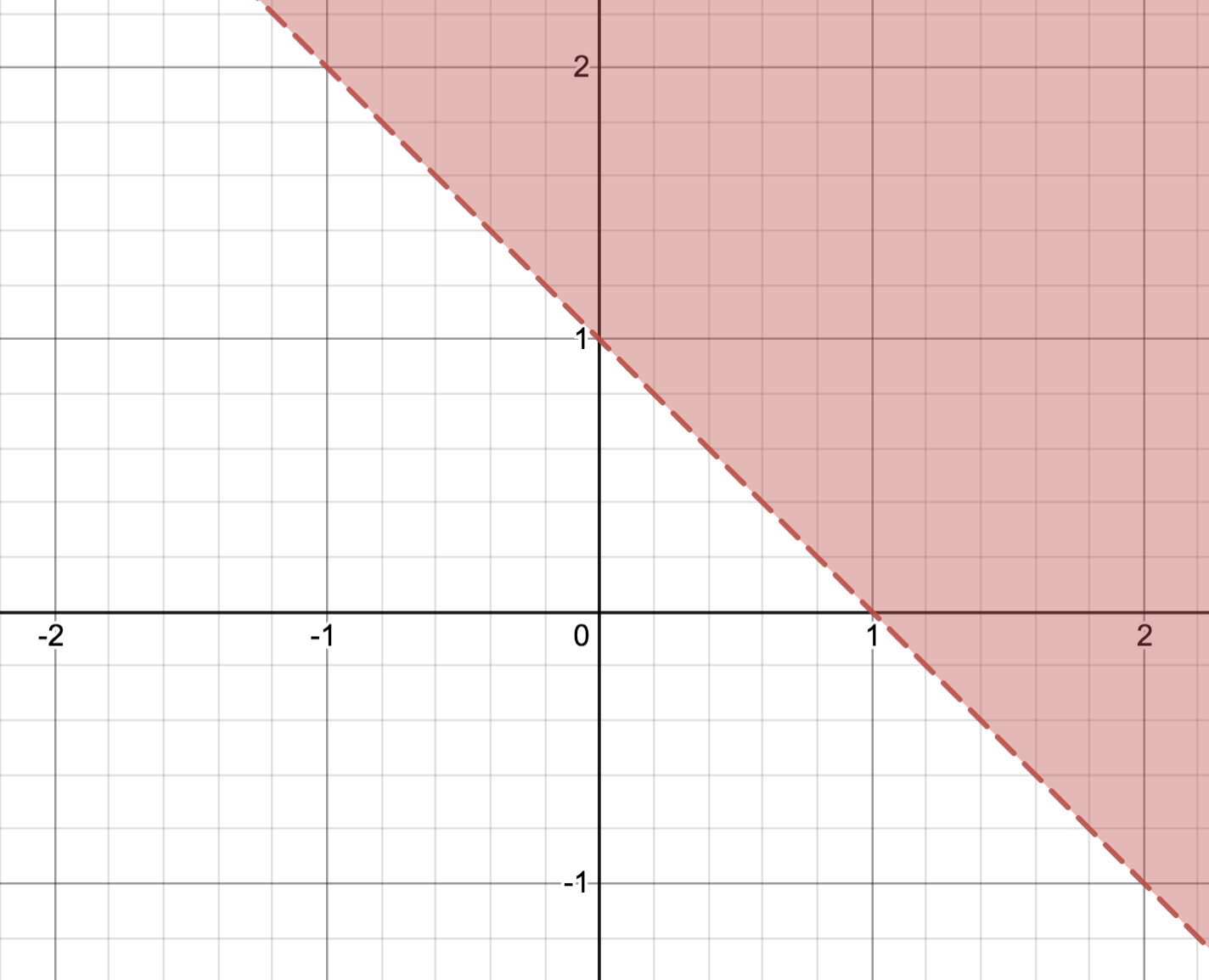
If we look at the graph we can see that (0, 0) is below the line and (2, 0) is above the line. Let’s use these to try to determine the different equations.

Solving for X

Given:

\[ \begin{aligned} w_y &= 1 \\ w_{bias} &= -1 \end{aligned} \]

and:

becomes

\[ \begin{aligned} loss_0 &= \left( \frac{1}{1 + e^{-w_x \cdot x - y + 1}} \right)^2 \\ loss_1 &= \left( \frac{1}{1 + e^{-w_x \cdot x - y + 1}} - 1 \right)^2 \end{aligned} \]

with the data points:

x	y	label
0	0	0
2	0	1

(varying only in x because that’s what we want to work out)

Then it becomes:

\[ \begin{aligned} loss &= \frac{1}{2}\left( \frac{1}{1 + e^{-w_x \cdot x - y + 1}} \right)^2 + \frac{1}{2}\left( \frac{1}{1 + e^{-w_x \cdot x - y + 1}} - 1 \right)^2 \\ loss &= \frac{1}{2}\left( \frac{1}{1 + e^{-w_x \cdot 0 - 0 + 1}} \right)^2 + \frac{1}{2}\left( \frac{1}{1 + e^{-w_x \cdot 2 - 0 + 1}} - 1 \right)^2 \\ loss &= \frac{1}{2}\left( \frac{1}{1 + e^1} \right)^2 + \frac{1}{2}\left( \frac{1}{1 + e^{-w_x \cdot 2 + 1}} - 1 \right)^2 \\ loss &= \frac{1}{2}\left( \frac{1}{1 + e} \right)^2 + \frac{1}{2}\left( \frac{1}{1 + e^{-w_x \cdot 2 + 1}} - 1 \right)^2 \\ \end{aligned} \]

So we can try plotting this on wolfram alpha to see the minimum.

The wolfram alpha equivalent equation is:

(0.5 * (1 / (1 + e))^2) + (0.5 * ((1 / (1 + e^(-2x + 1))) - 1)^2)

Which ends up being this:

https://www.wolframalpha.com/input/?i=minimize+%280.5++%281+%2F+%281+%2B+e%29%29%5E2%29+%2B+%280.5++%28%281+%2F+%281+%2B+e%5E%28-2x+%2B+1%29%29%29+-+1%29%5E2%29

Which has no global minima. Bah.

I don’t think I should be surprised by this - x only appears on one side of the equation.

So to make this easier I could try plotting in the notebook. The first thing to do is to be able to generate the different points on the graph.

Code

from typing import *
from math import e

def generate_points(equation: str) -> Tuple[List[float], List[float]]:
    generator = eval(f"lambda v: {equation}")
    x = [(i / 10) for i in range(-20, 20)]
    y = [
        generator(i)
        for i in x
    ]
    return x, y

Code

import matplotlib.pyplot as plt

def show_graph(x: List[float], y: List[float]) -> None:
    plt.figure()
    plt.plot(x, y)

Code

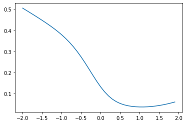
show_graph(*generate_points("(0.5 * (1 / (1 + e))**2) + (0.5 * ((1 / (1 + e**(-2*v + 1))) - 1)**2)"))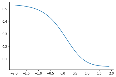

It’s turned into a sigmoid. As I said this isn’t hugely surprising.

Lets pick some non zero points.

Code

def to_equation(
    weight_x: Optional[float],
    weight_y: Optional[float],
    bias: Optional[float],
    x: float,
    y: float,
    label: int
) -> str:
    assert sum(v is None for v in [weight_x, weight_y, bias]) == 1
    
    if weight_x is None:
        weight_x = "v"
    if weight_y is None:
        weight_y = "v"
    if bias is None:
        bias = "v"

    return f"(1 / (1 + e**-({x}*{weight_x} + {y}*{weight_y} + {bias})) - {label})**2"

Code

to_equation(
    weight_x=None,
    weight_y=1,
    bias=-1,
    x=3,
    y=4,
    label=1,
)

'(1 / (1 + e**-(3*v + 4*1 + -1)) - 1)**2'

Code

show_graph(*generate_points(to_equation(
    weight_x=None,
    weight_y=1,
    bias=-1,
    x=3,
    y=4,
    label=1,
)))

Code

def combine(*equations) -> str:
    divisor = f"1/{len(equations)}"
    
    return " + ".join(
        f"{divisor}*{equation}"
        for equation in equations
    )

def show(equation: str) -> None:
    show_graph(*generate_points(equation))

Code

combine(
    to_equation(
        weight_x=None,
        weight_y=1,
        bias=-1,
        x=3,
        y=4,
        label=1,
    ),
    to_equation(
        weight_x=None,
        weight_y=1,
        bias=-1,
        x=-3,
        y=4,
        label=0,
    ),
)

'1/2*(1 / (1 + e**-(3*v + 4*1 + -1)) - 1)**2 + 1/2*(1 / (1 + e**-(-3*v + 4*1 + -1)) - 0)**2'

Code

show(combine(
    to_equation(
        weight_x=None,
        weight_y=1,
        bias=-1,
        x=1,
        y=1,
        label=1,
    ),
    to_equation(
        weight_x=None,
        weight_y=1,
        bias=-1,
        x=-1,
        y=1,
        label=0,
    ),
))

Code

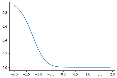
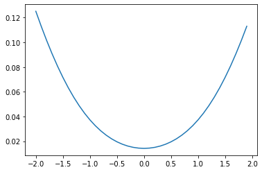
show(combine(
    *[
        to_equation(
            weight_x=None,
            weight_y=1,
            bias=-1,
            x=x,
            y=y,
            label=label,
        )
        for x, y, label in [
            (-1, 1, 0),
            (1, -1, 0),
            (3, 1, 1),
            (1, 3, 1),
        ]
    ]
))

I finally have it. Here I chose points that form a cross around a division point on the line. It looks like it has a minima around 1.0.

I wonder if I was choosing the wrong dimension to vary all along?

Code

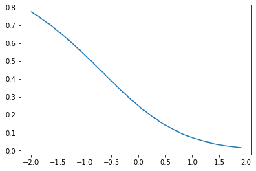
show(combine(
    *[
        to_equation(
            weight_x=None,
            weight_y=1,
            bias=-1,
            x=x,
            y=y,
            label=label,
        )
        for x, y, label in [
            (1, -1, 0),
            (1, 3, 1),
        ]
    ]
))

This also clearly has a minima. The fun thing is this is not wrong - there are an infinite number of lines that divide two points. This has chosen the line with \(y = 0\).