I want to understand how quantum circuits work. Since I’ve got a programming background I’m more interested in the underlying implementation in classical computing as that will allow me to translate the quantum computing knowledge into a domain I already understand.
I got annoyed with the QuTiP framework however that exposed the underlying operations as matrix operations. That helps me quite a bit. Maybe looking into the matrix representation of the Qiskit gates would be productive?
Youtube Interlude
I’ve actually found this video extremely helpful:
youtube: https://youtu.be/wLv20RHqlgw
It’s part of a series on quantum computing.
This video explains that a quantum gate is more easily understood than classical quantum computing because we can limit the effect of any operation to a small number of qubits. It starts with the NOT gate.
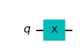
NOT Gate
This inverts the qubit which can be expressed as:
\[ \left| 0 \right\rangle \rightarrow \left| 1 \right\rangle \\ \left| 1 \right\rangle \rightarrow \left| 0 \right\rangle \]
And this can be expressed as the [x] operator which turned up a lot in the diagrams from the qiskit evaluation:
This is a linear transformation. All quantum gates are unitary transformations which means that:
- They must be reversible
- They preserve the inner product
The inner product requirement is a bit difficult to understand for me. As I understand it, the inner product is being taken between the vector and itself. The inner product is defined as $ (a,b) = |a||b| $. To show that this rule can be violated can we produce two vectors that have a different inner product with themselves?
Since they are being compared with themselves the angle between the two vectors is zero. \(\cos(0) = 1\) so we can drop the cosine part.
The other part can be expanded as:
\[ |a||b| = a_1 b_1 + a_2 b_2 + ... + a_n b_n \]
Which is the dot product. Coming up with two vectors that have a different dot product is easy:
Code
import numpy as np

a = np.array([1, 0])
b = np.array([0.5, 0.5])

np.dot(a, a), np.dot(b, b)
(1, 0.5)So Quantum Gate operations preserve the dot product of the vector with itself. This is explained as the state representing a point on the qubit surface and thus needing to be normalized:
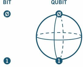
This means that my initial use of the QiTiP framework could not be represented as a qubit. I initialized it with the array [1, 2, 3] which is not normalized. I feel like I have chosen the correct framework to work within.
This leads to an insight into how the NOT gate can be reversible. If we want to invert the qubit then we must “push” the value that it has into another dimension (which would then be reversible, as we could “pull” the value back). The computation is thus the measurement of a single dimension of the qubit which does not need to satisfy the inner product on it’s own.
This conclusion is reinforced by the matrix representation of the NOT gate:
\[ \hat{x} = \begin{pmatrix} 0 & 1 \\ 1 & 0 \\ \end{pmatrix} \]
Where the two columns of the matrix represent \(\left| 0 \right\rangle\) and \(\left| 1 \right\rangle\).
I want to be able to visualize the circuits that I am going to use to explore the different behaviours of quantum circuits. We will also explore the probabilistic nature of quantum computing, so we must show the results of different runs. To do this I am using the following code:
Code
from qiskit import QuantumCircuit
from qiskit.result.result import Result
from qiskit.visualization import plot_histogram

def show_results(qc: QuantumCircuit, shots: int = 1024) -> Result:
    # execute is a super generic term
    from qiskit import Aer, execute

    backend = Aer.get_backend('qasm_simulator')
    job = execute(qc, backend, shots=shots, memory=True)
    output = job.result()

    display(qc.draw(output="mpl"))
    display(
        plot_histogram(output.get_counts(qc))
    )
    return output
Hadamard Gate and Superpositions
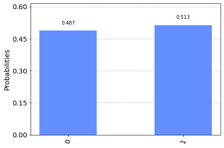
The Hadamard gate is interesting because it puts the qubit into a superposition state. In practice this means that the value when measured is non deterministic, either being \(\left| 0 \right\rangle\) or \(\left| 1 \right\rangle\). This seems like an excellent way to introduce randomness into the circuit.
The Hadamard gate is it’s own inverse, so if we pass a fixed qubit through two of them we get the original value.
You can see this in the two simulations below:
Code
from qiskit import QuantumCircuit

qc = QuantumCircuit(1, 1)
qc.reset(0)

qc.h(0)

qc.measure(0,0)

result = show_results(qc)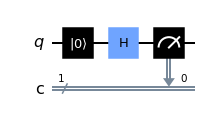
Code
from qiskit import QuantumCircuit

qc = QuantumCircuit(1, 1)
qc.reset(0)

qc.h(0)
qc.h(0)

qc.measure(0,0)

result = show_results(qc)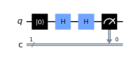

I find this gate really interesting as it shows that the process of measurement restricts the available values.
There is one further subtlety of the Hadamard gate. Is inverting the qubit before running two Hadamard gates (-[x]-[h]-[h]-) equivalent to inverting the qubit in between the two Hadamard gates (-[h]-[x]-[h]-)?
Code
from qiskit import QuantumCircuit

qc = QuantumCircuit(1, 1)
qc.reset(0)

qc.x(0)
qc.h(0)
qc.h(0)

qc.measure(0,0)

result = show_results(qc)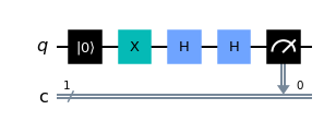

Code
from qiskit import QuantumCircuit

qc = QuantumCircuit(1, 1)
qc.reset(0)

qc.h(0)
qc.x(0)
qc.h(0)

qc.measure(0,0)

show_results(qc)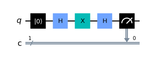

We can see that it is not, -[x]-[h]-[h]- is \(\left| 1 \right\rangle\) and -[h]-[x]-[h]- is \(\left| 0 \right\rangle\). Why do they differ?
In the first experiment we put the qubit in the \(\left| 1 \right\rangle\) state, by applying [x], and put it through two Hadamard gates. As expected the result is \(\left| 1 \right\rangle\), because the Hadamard gate is it’s own inverse.
When we apply the [x] operator between the two Hadamard gates then we get the value \(\left| 0 \right\rangle\). The video explains that the Hadamard gate puts the \(\left| 0 \right\rangle\) qubit into the state \(\frac{1}{\sqrt{x}} \left( \left| 0 \right\rangle + \left| 1 \right\rangle \right)\), which when inverted becomes \(\frac{1}{\sqrt{x}} \left( \left| 1 \right\rangle + \left| 0 \right\rangle \right)\). The inverted form is equal to the original so the application of [x] has had no effect.
It’s interesting that the prior application of [x] results in the value of \(\left| 1 \right\rangle\) being preserved. This is because the Hadamard gate when applied to \(\left| 1 \right\rangle\) results in \(\frac{1}{\sqrt{x}} \left( \left| 0 \right\rangle - \left| 1 \right\rangle \right)\) (note the minus sign).
Controlled NOT Gate (XOR)
This inverts the qubit, if the control qubit is in the \(\left| 1 \right\rangle\) state, which can be expressed as:
\[ \left| 0 0 \right\rangle \rightarrow \left| 0 0 \right\rangle \\ \left| 0 1 \right\rangle \rightarrow \left| 0 1 \right\rangle \\ \left| 1 0 \right\rangle \rightarrow \left| 1 1 \right\rangle \\ \left| 1 1 \right\rangle \rightarrow \left| 1 0 \right\rangle \]
We saw this used as the XOR gate in the initial evaluation of this framework.
When this is represented as a matrix it is shown as:
\[ \begin{pmatrix} 1 & 0 & 0 & 0 \\ 0 & 1 & 0 & 0 \\ 0 & 0 & 0 & 1 \\ 0 & 0 & 1 & 0 \end{pmatrix} \]
This was a revelation to me as it shows that each column of the matrix is really just a specific state of the two qubits and that the column then defines the resulting state. I feel that this is not matrix multiplication as I previously understood it - this 4x4 matrix is describing the transformation of a pair of qubits.
I am now recalling that the original NOT gate was a 2x2 matrix, and so each qubit has two values within it. That makes a bit more sense.
We could explore the equivalence between this and regular matrix multiplication though:
Code
from IPython.display import Latex
import numpy as np

qstate = [
    [0, 1], # |0>
    [1, 0], # |1>
]
qstate_inverse = {
    (0, 1): 0,
    (1, 0): 1,
}
cnot = np.array([
    [1, 0, 0, 0],
    [0, 1, 0, 0],
    [0, 0, 0, 1],
    [0, 0, 1, 0],
])

for x, y in [
    [0,0],
    [0,1],
    [1,0],
    [1,1],
]:
    in_matrix = np.array(qstate[x] + qstate[y])
    out_matrix = in_matrix @ cnot
    x_out = qstate_inverse[(out_matrix[0], out_matrix[1])]
    y_out = qstate_inverse[(out_matrix[2], out_matrix[3])]
    print(f"|{x}{y}> -> |{x_out}{y_out}>")
|00> -> |01>
|01> -> |00>
|10> -> |11>
|11> -> |10>I think I did this correctly? It does not match the result of the application of the gate (mapping of \(\left| 0 1 \right\rangle\) is incorrect). This does feel like a revelation regarding the matrix representation of quantum gates.
Controlled NOT Gate and Superpositions
An interesting application of the CNOT gate is to apply it using a control qubit in the superposition state. Let’s start by considering what we get if two qubits are in the superposition state:
Code
from qiskit import QuantumCircuit

qc = QuantumCircuit(2, 2)
qc.reset(0)
qc.reset(1)

qc.h(0)
qc.h(1)

qc.measure([0,1],[0,1])

show_results(qc)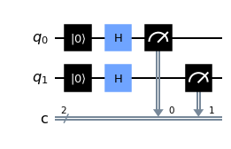
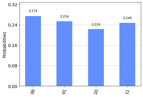
We can see here that we get all 4 possible outcomes approximately equally.
If we use CNOT with a superposition qubit as the control qubit what happens? Thinking this through - if the control qubit is set then the target qubit should be inverted. If the control qubit is not set then the target qubit should not be inverted. However we do not know the state of the control qubit until it is measured:
Code
from qiskit import QuantumCircuit

qc = QuantumCircuit(2, 2)
qc.reset(0)
qc.reset(1)

qc.h(0)
qc.cx(control_qubit=0, target_qubit=1)

qc.measure([0,1],[0,1])

show_results(qc)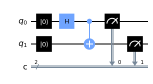
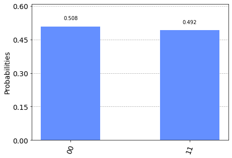
We can see that this has ensured that the two qubits share the same state. Apparently this is the quantum entanglement that I have heard so much about.
Since it is the inversion which is controlled, we can flip the target qubit before entangling them to ensure that they never share the same state:
Code
from qiskit import QuantumCircuit

qc = QuantumCircuit(2, 2)
qc.reset(0)
qc.reset(1)

qc.h(0)
qc.x(1)
qc.cx(control_qubit=0, target_qubit=1)

qc.measure([0,1],[0,1])

show_results(qc)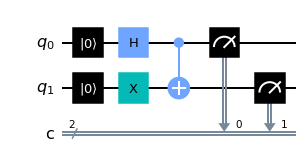
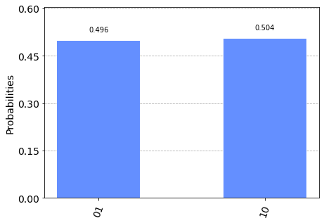
This is great! We can now choose between two different values using this technique.
What would be required to extend this to three different values?
Superposition Probability Distribution
To choose between three different values it would be easy if we can have a \(\frac{1}{3}\) probability for an individual qubit. Since we have a way to produce the 50/50 distribution, reviewing how the Hadamard gate works might provide a hint for producing a different distribution.
The matrix representation of the Hadamard gate is:
\[ H = \frac{1}{\sqrt{2}} \begin{pmatrix} 1 & 1 \\ 1 & -1 \\ \end{pmatrix} \]
This means that the \(\left| 0 \right\rangle\) and \(\left| 1 \right\rangle\) values are mapped to their superpositions as follows:
\[ \begin{align} \left| 0 \right\rangle &\rightarrow \begin{bmatrix} \frac{1}{\sqrt{2}} & \frac{1}{\sqrt{2}} \end{bmatrix} \\ \left| 1 \right\rangle &\rightarrow \begin{bmatrix} \frac{1}{\sqrt{2}} & -\frac{1}{\sqrt{2}} \end{bmatrix} \end{align} \]
If we plot the values of \(\left| 0 \right\rangle\), \(\left| 1 \right\rangle\) and the associated superpositions then we might see something interesting.
Code
import math
import pandas as pd

df = pd.DataFrame([
    {"state": "0", "x": 0, "y": 1},
    {"state": "1", "x": 1, "y": 0},
    {"state": "superposition-0", "x": 1/math.sqrt(2), "y": 1/math.sqrt(2)},
    {"state": "superposition-1", "x": 1/math.sqrt(2), "y": -1/math.sqrt(2)},
])
df.plot.scatter(
    x="x",
    y="y",
    # force it into a square to better show the shape
    figsize=(4,4),
    xlim=(-1.1,1.1),
    ylim=(-1.1,1.1)
)
df| state | x | y | |
|---|---|---|---|
| 0 | 0 | 0.000000 | 1.000000 |
| 1 | 1 | 1.000000 | 0.000000 |
| 2 | superposition-0 | 0.707107 | 0.707107 |
| 3 | superposition-1 | 0.707107 | -0.707107 |
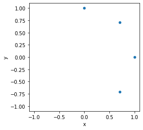
If we squint then it should be possible to make out a circle forming from these points. Remembering that the values of the qubit form a shell we should see that this is the unit circle. This is because the inner product is preserved:
Code
import numpy as np
import math

a = np.array([1, 0])
b = np.array([1/math.sqrt(2), 1/math.sqrt(2)])

np.dot(a,a), round(np.dot(b,b), 3)
(1, 1.0)We can see that using \(\frac{1}{\sqrt{2}}\) as the value for both x and y preserves the inner product.
Entering Superpositions
There are several different ways to enter a super position, which I will run through now.
Qubit Initialization
The first is to initialize the qubit into the superposition:
Code
from qiskit import QuantumCircuit
import math

qc = QuantumCircuit(1, 1)
qc.initialize(
    [
        math.sqrt(x)
        for x in [1/2, 1/2]
    ]
)

qc.measure(0, 0)

output = show_results(qc)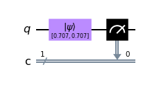

To do this correctly we must square root the values because the probability distribution is defined in terms of the ratio between x and y. This ratio is expressed here: for x in [1/2, 1/2]
The initialization of the qubit requires that the sum of squares be equal to 1, which we can see below:
Code
from qiskit import QuantumCircuit

qc = QuantumCircuit(1, 1)
qc.initialize(
    [1/2, 1/2]
)
QiskitError: 'Sum of amplitudes-squared does not equal one.'This initialization is really easy as we can specify the probability distribution directly. It would be nice to have a way to conditionally leave the superposition, so is there a way that works with control qubits?
Rotation Gate
Reviewing the Qiskit API, I find the RGate and RXGate which can rotate the qubit. This takes a theta value which corresponds to the rotation angle. The relationship between this angle and the probability distribution is not linear:
Code
from qiskit.circuit.library.standard_gates.rx import RXGate
import math
import numpy as np
import pandas as pd

def expected_probability(rotation: float) -> float:
    gate = RXGate(theta=rotation)
    probability = gate.__array__()[0, 0]**2
    # it's a complex number, but the imaginary part is zero
    return np.round(1 - probability, 3).real

df = pd.DataFrame([
    {
        "rotation": math.pi * numerator / 20,
        "probability": expected_probability(math.pi * numerator / 20),
    }
    for numerator in range(20)
]).set_index("rotation")

df.plot() ; None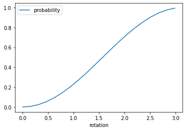
We can see that these values correspond to the probability distributions by running each one through:
Code
import math
import pandas as pd

def observed_probability(rotation: float) -> float:
    from qiskit import QuantumCircuit, Aer, execute

    qc = QuantumCircuit(1, 1)
    qc.reset(0)
    qc.rx(theta=rotation, qubit=0)
    qc.measure(0, 0)

    backend = Aer.get_backend('qasm_simulator')
    job = execute(qc, backend, shots=10_000, memory=True)
    output = job.result()
    counts = output.get_counts()
    actual_probability = (
        counts.get("1", 0) / (counts.get("0", 0) + counts.get("1", 0))
    )

    return round(actual_probability, 3)

df = pd.DataFrame([
    {
        "rotation": rotation,
        "expected": expected_probability(rotation),
        "observed": observed_probability(rotation),
        "cosine": (-math.cos(rotation) + 1)/2,
    }
    for rotation in [v*math.pi/20 for v in range(20)]
]).set_index("rotation")

df.plot()
df| expected | observed | cosine | |
|---|---|---|---|
| rotation | |||
| 0.000000 | 0.000 | 0.000 | 0.000000 |
| 0.157080 | 0.006 | 0.006 | 0.006156 |
| 0.314159 | 0.024 | 0.024 | 0.024472 |
| 0.471239 | 0.054 | 0.055 | 0.054497 |
| 0.628319 | 0.095 | 0.097 | 0.095492 |
| 0.785398 | 0.146 | 0.146 | 0.146447 |
| 0.942478 | 0.206 | 0.209 | 0.206107 |
| 1.099557 | 0.273 | 0.271 | 0.273005 |
| 1.256637 | 0.345 | 0.344 | 0.345492 |
| 1.413717 | 0.422 | 0.429 | 0.421783 |
| 1.570796 | 0.500 | 0.507 | 0.500000 |
| 1.727876 | 0.578 | 0.580 | 0.578217 |
| 1.884956 | 0.655 | 0.652 | 0.654508 |
| 2.042035 | 0.727 | 0.734 | 0.726995 |
| 2.199115 | 0.794 | 0.788 | 0.793893 |
| 2.356194 | 0.854 | 0.852 | 0.853553 |
| 2.513274 | 0.905 | 0.906 | 0.904508 |
| 2.670354 | 0.946 | 0.948 | 0.945503 |
| 2.827433 | 0.976 | 0.977 | 0.975528 |
| 2.984513 | 0.994 | 0.995 | 0.993844 |
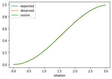
You can see that the array representation of the gate is strongly correlated with the observed probability distribution, and that the relationship is not linear. This is not surprising as it is related to trigonometry, and we are actually observing a cosine wave.
This means that to produce a specific probability distribution we need to use the inverse cosine. In our demonstration, above, we used the equation \(P = \frac{\cos(\theta) + 1}{2}\). To calculate the angle required for a given probability we just have to invert it. Because I’m a math scrub I’m going to write this out step by step:
\[ \begin{aligned} P &= \frac{1 - \cos(\theta)}{2} \\ 2 P &= 1 - \cos(\theta) \\ 2 P - 1 &= -\cos(\theta) \\ -(2 P - 1) &= \cos(\theta) \\ \arccos(-(2 P - 1)) &= \theta \end{aligned} \]
We can check our work by running this over specific probabilities:
Code
import math
import pandas as pd

def to_rotation(probability: float) -> float:
    return math.acos(-(probability * 2 - 1))

df = pd.DataFrame([
    {
        "probability": probability,
        "expected": expected_probability(to_rotation(probability)),
        "observed": observed_probability(to_rotation(probability)),
    }
    for probability in [v/20 for v in range(20)]
]).set_index("probability")

df.plot()
df| expected | observed | |
|---|---|---|
| probability | ||
| 0.00 | 0.00 | 0.000 |
| 0.05 | 0.05 | 0.050 |
| 0.10 | 0.10 | 0.104 |
| 0.15 | 0.15 | 0.144 |
| 0.20 | 0.20 | 0.198 |
| 0.25 | 0.25 | 0.254 |
| 0.30 | 0.30 | 0.303 |
| 0.35 | 0.35 | 0.353 |
| 0.40 | 0.40 | 0.399 |
| 0.45 | 0.45 | 0.446 |
| 0.50 | 0.50 | 0.500 |
| 0.55 | 0.55 | 0.553 |
| 0.60 | 0.60 | 0.599 |
| 0.65 | 0.65 | 0.648 |
| 0.70 | 0.70 | 0.696 |
| 0.75 | 0.75 | 0.751 |
| 0.80 | 0.80 | 0.796 |
| 0.85 | 0.85 | 0.853 |
| 0.90 | 0.90 | 0.899 |
| 0.95 | 0.95 | 0.949 |
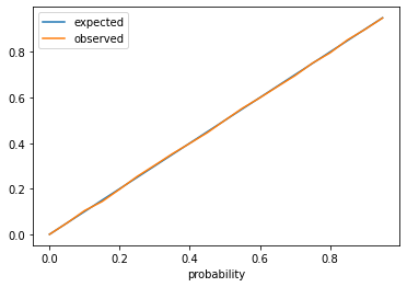
Using rotation with qubits is better than initialization because we can move out of the superposition as easily as we moved into it. With this we can see that the Hadamard gate is a specific rotation that has a probability of 0.5.
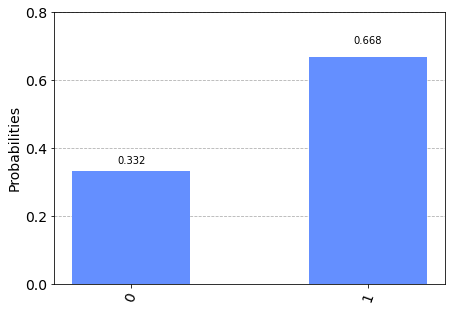
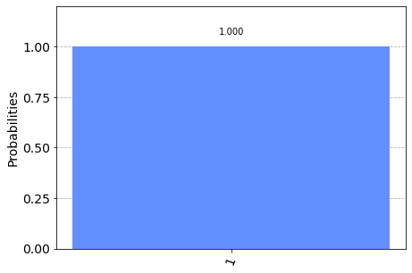
To see if rotation out of a superposition works we can review what the distribution looks like after the initial rotation:
Code
from qiskit import QuantumCircuit
import math

qc = QuantumCircuit(1, 1)

qc.rx(theta=to_rotation(2/3), qubit=0)
qc.measure(0, 0)

output = show_results(qc, shots=10_000)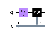
And then try rotating further to the \(\left| 1 \right\rangle\) state:
Code
from qiskit import QuantumCircuit
import math

qc = QuantumCircuit(1, 1)

qc.rx(theta=to_rotation(2/3), qubit=0)
qc.rx(theta=to_rotation(1/3), qubit=0)
qc.measure(0, 0)

output = show_results(qc, shots=10_000)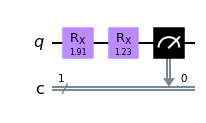
3 Bit Chooser
To have an even three way choice we can define the following:
- The first bit is chosen with probability 1/3.
- IFF the first bit is not chosen then the second is chosen with probability 1/2.
- IFF the first and second bits are not chosen then the third is chosen.
We can express this by turning off the subsequent bits by conditionally rotating them. The two implementations that follow show that the Hadamard gate can be replaced with a rotation:
Code
from qiskit import QuantumCircuit
import math
qc = QuantumCircuit(3, 3)
qc.rx(theta=to_rotation(1/3), qubit=0)
# Using Hadamard here
qc.h(qubit=1)
qc.x(qubit=2)
# turn off 1 and 2 if 0 is set
# Using conditional Hadamard here
qc.ch(control_qubit=0, target_qubit=1)
qc.cx(control_qubit=0, target_qubit=2)
# turn off 2 if 1 is set (exclusive with above due to order)
qc.cx(control_qubit=1, target_qubit=2)
qc.measure([0,1,2], [0,1,2])
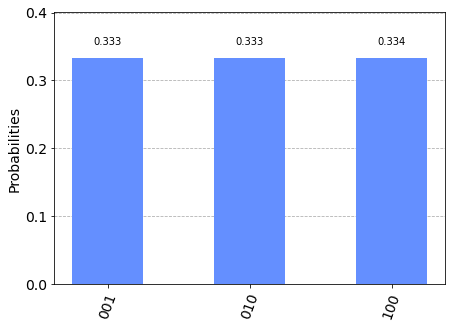
output = show_results(qc, shots=100_000)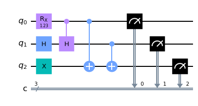
Code
from qiskit import QuantumCircuit
import math

qc = QuantumCircuit(3, 3)

qc.rx(theta=to_rotation(1/3), qubit=0)
# Using rotation here
qc.rx(theta=to_rotation(1/2), qubit=1)
qc.x(qubit=2)

# turn off 1 and 2 if 0 is set
# Using rotation here
qc.crx(theta=to_rotation(1/2), control_qubit=0, target_qubit=1)
qc.cx(control_qubit=0, target_qubit=2)

# turn off 2 if 1 is set (exclusive with above due to order)
qc.cx(control_qubit=1, target_qubit=2)

qc.measure([0,1,2], [0,1,2])

output = show_results(qc, shots=100_000)
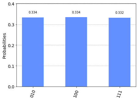
I’m pretty happy with this distribution - the variance between the observed values and the ideal values is extremely small. Furthermore the two circuits are equivalent when measured, showing that Hadamard gates can be replaced with rotation.
N Bit Chooser
The best thing about this approach is that we can then extend it to a four way chooser. All we need to do is add another control bit that is rotated with probability \(\frac{1}{4}\):
Code
from qiskit import QuantumCircuit
import math

qc = QuantumCircuit(4, 4)

quarter_rotation = to_rotation(1/4)
third_rotation = to_rotation(1/3)

qc.rx(theta=quarter_rotation, qubit=0)
qc.rx(theta=third_rotation, qubit=1)
qc.h(qubit=2)
qc.x(qubit=3)

# turn off 1, 2 and 3 if 0 is set
qc.crx(theta=-third_rotation, control_qubit=0, target_qubit=1)
qc.ch(control_qubit=0, target_qubit=2)
qc.cx(control_qubit=0, target_qubit=3)

# turn off 2 and 3 if 1 is set
qc.ch(control_qubit=1, target_qubit=2)
qc.cx(control_qubit=1, target_qubit=3)

# turn off 3 if 2 is set (exclusive with above due to order)
qc.cx(control_qubit=2, target_qubit=3)

qc.measure([0,1,2,3], [0,1,2,3])

output = show_results(qc, shots=100_000)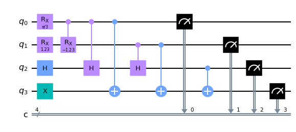
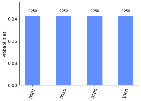
This algorithm can be extended to choose between any number of bits by just adding more control bits. Here we define a fully generic chooser:
Code
from qiskit import QuantumCircuit
import math

def nway_chooser(n: int) -> QuantumCircuit:
    assert n >= 4

    qc = QuantumCircuit(n, n)

    rotations = {
        v: to_rotation(1/(n-v))
        for v in range(n)
    }

    for qubit, rotation in rotations.items():
        qc.rx(theta=rotation, qubit=qubit)

    for control_qubit in range(n):
        for target_qubit in range(control_qubit+1, n):
            target_rotation = rotations[target_qubit]
            qc.crx(
                theta=-target_rotation,
                control_qubit=control_qubit,
                target_qubit=target_qubit
            )
        if control_qubit+1 < n:
            qc.barrier() # makes it render nicely

    qc.measure(range(n), range(n))

    return qc
Code
qc = nway_chooser(5)
show_results(qc, shots=1_000_000) ; None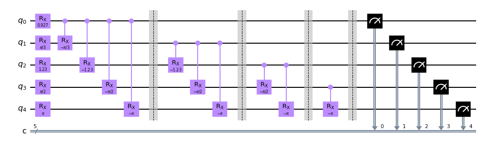
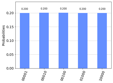
Here to make the programming easier I am using the RXGate for everything, including places where the plain XGate or HGate could be used. I think this is a huge success and I see no reason why this couldn’t extend to an arbitrary number of qubits. Great stuff.
To improve this would require having a gate that could set many qubits based on a single control bit. The repeating pattern in this algorithm is setting every qubit below the current one if the comparison passes. Being able to do that in a single operation would make the visualization more compact. I have not seen a way to define an arbitrary gate in Qiskit though.