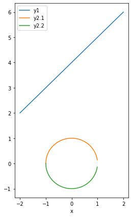
import pandas as pdimport numpy as npdf = pd.DataFrame( np.arange(-2, 2.01, 0.01), columns=["x"]).set_index("x")# first equation, y = x + 4df["y1"] = df.index +4# second equation x^2 + 2y^2 = 1# the second equation is done over two series to handle the + and the -df["y2.1"] = (1-df.index**2)**0.5df["y2.2"] =-(1-df.index**2)**0.5df.plot(figsize=(4,7)) ;None
The orange and green lines both form the \(x^2 + 2y^2 = 1\) line. The gap in the circle is caused by plotting the curves as a collection of discrete points.
In my poor plot of these equations we can see that there is no perfect point that satisfies both equations. Instead we should find the point that minimizes the distance between the points. I can restrict the second equation to only the positive values and then it should be possible to write an equation for the distance between the lines.
The distance between the lines is the difference between these two equations:
\[
\begin{aligned}
y &= x + 4 \\
y &= \sqrt{\frac{1 - x^2}{2}}
\end{aligned}
\]
We can express this as:
\[
distance = x + 4 - \sqrt{\frac{1 - x^2}{2}}
\]
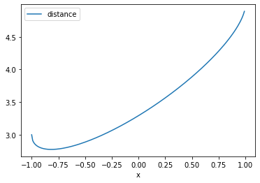
And plotting this:
Code
import pandas as pdimport numpy as npdf = pd.DataFrame( np.arange(-1, 1.01, 0.01), columns=["x"]).set_index("x")df["distance"] = df.index +4- ((1- df.index**2) /2)**0.5df.plot() ;None
We can see that the minimum distance is between -1 and -0.75. It should be possible to find the point by calculating the derivative of this equation. Wolfram Alpha tells me that it is
The above problem was then extended to finding the probability distribution that best fits a weighted die that has an average roll of 4.5. The best probabilistic model is the one that maximizes the entropy. This is the best because it applies the least constraint over the system - a system with lower entropy is more predictable.
We can define the entropy of the model b with:
\[
H(\text{p}) = -\sum_i{p_i \log p_i}
\]
Our model is that a 6 sided die has an average roll of 4.5. That can be expressed as two equations:
The first establishes that the total probability across the different outcomes sums to one, which means we arn’t dealing with a die with a different shape. The second expresses the average value that is rolled is a 4.5.
We can then calculate the differential of all of these based on two simple facts:
\[
\frac{d}{dx} x = 1
\]
and
\[
\frac{d}{dx} x \log x = \log x + 1
\]
That means we can state the differentials of the equations as:
\[
p = (0.054, 0.079, 0.114, 0.165, 0.24, 0.347)
\]
The problem here isn’t the problem specification, it’s the method of solving it…
The hard problem is to solve this using pure pytorch. To do this we have to think about how pytorch works.
Optimization Approach
The first way that I would solve this problem is to define the two variables, \(\lambda\) and \(\mu\) as pytorch parameters and then define a loss function which measures how closely they adhere to the constraints. This would involve defining the value of \(p_1, \ldots, p_6\) in terms of those two variables and then finding the distance from the correct value for functions f and g.
Using absolute in a loss function is generally discouraged because it is discontinuous at zero. Instead I will square the value to ensure it remains positive and continuous. That leads to a final pair of loss functions:
#collapsefrom typing import Tupleimport torchfrom torch import nn# The six probabilities corresponding to p1,...,p6Answer = Tuple[float, float, float, float, float, float]class LambdaMuOptimizer(nn.Module):def__init__(self, average_roll: float, lambda_: float, mu: float ) ->None:super().__init__()self.average_roll = average_rollself.lambda_ = torch.nn.Parameter(torch.tensor(lambda_))self.mu = torch.nn.Parameter(torch.tensor(mu))def optimize(self, iterations: int=10_000) -> Answer: df =self.train(iterations)# Show how the loss has changed over the training df[["loss"]].plot(logy=True)# Find the best performing row and show it best_row = df[df.loss == df.loss.min()]print(best_row)# Then calculate and return the different probabilitiesreturnself.ps().tolist()def train(self, iterations: int, lr: float=0.01) ->None: optimizer = torch.optim.AdamW(self.parameters(), lr=lr) steps = []for _ inrange(iterations): optimizer.zero_grad() loss =self.loss() steps.append(( loss.item(),self.lambda_.item(),self.mu.item() )) loss.backward() optimizer.step()return pd.DataFrame(steps, columns=["loss", "𝜆", "𝜇"])def loss(self) -> torch.Tensor: ps =self.ps()returnself.loss_f(ps) +self.loss_g(ps, self.average_roll)@staticmethoddef loss_f(ps: torch.Tensor) -> torch.Tensor:return (ps.sum() -1)**2@staticmethoddef loss_g(ps: torch.Tensor, target_average_roll: float) -> torch.Tensor: average_roll = (ps * torch.tensor([1, 2, 3, 4, 5, 6])).sum()return (average_roll - target_average_roll)**2def ps(self) -> torch.Tensor:return torch.cat([self.p1()[None],self.p2()[None],self.p3()[None],self.p4()[None],self.p5()[None],self.p6()[None], ], dim=0)def pn(self, n: int) -> torch.Tensor:# These calculate the value of p1,...,p6 given 𝜆 and 𝜇 exponent =-(self.lambda_ + (n *self.mu) +1)return torch.exp(exponent)def p1(self) -> torch.Tensor:returnself.pn(1)def p2(self) -> torch.Tensor:returnself.pn(2)def p3(self) -> torch.Tensor:returnself.pn(3)def p4(self) -> torch.Tensor:returnself.pn(4)def p5(self) -> torch.Tensor:returnself.pn(5)def p6(self) -> torch.Tensor:returnself.pn(6)
Code
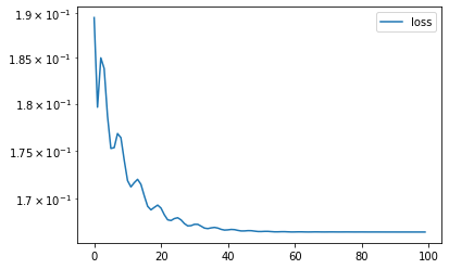
model = LambdaMuOptimizer( average_roll=4.5, lambda_=0.15, mu=0.15)probabilities = model.optimize(iterations=10_000)total_probability =sum(probabilities)average_roll =sum( value * probabilityfor value, probability inenumerate(probabilities, start=1))print(f"Probabilities sum to: {total_probability:0.5f}")print(f"Average roll is: {average_roll:0.5f}")probabilities
          loss         𝜆        𝜇
9676  0.000071  2.200761 -0.35447
Probabilities sum to: 1.00832
Average roll is: 4.49824
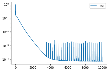
With 10,000 iterations and a sophisticated optimizer we can arrive at values which are approximately correct. The correct values are:
\[
p=(0.054,0.079,0.114,0.165,0.24,0.347)
\]
and this has produced
\[
p=(0.058,0.083,0.118,0.168,0.24,0.342)
\]
which is close but is not completely correct. The loss curve also shows that the progress towards the correct solution became very noisy towards the end.
Manifold Approach
Optimising over 𝜆 and 𝜇 is difficult because the constraints of \(\sum_i p_i = 1\) and \(\sum_i i p_i = 4.5\) get broken as the values change. Defining those constraints as loss functions means that the solution can move close to them but they are never likely to be satisfied. This is because the loss gets smaller and smaller as it moves towards satisfying them.
Instead we could try to parameterize the “model” in terms of the p values and then calculate the loss according to how well the points lie on the line defined by 𝜆 and 𝜇. The two equations are linear with respect to the inputs so it should be possible to map any set of values to the nearest point which satisfies both equations.
To practice this lets imagine that we are dealing with a 4 sided die instead (which will now average 2.5). This way there will be two degrees of freedom as the two constraints should result in a balance. If we randomly set \(p_1\) and \(p_4\) then it should be easy to see that \(p_2 = p_4\) and \(p_3 = p_1\) in order to maintain \(\sum_i i p_i = 2.5\). Then normalizing the values would satisfy the \(\sum_i p_i = 1\).
That is a well defined way to satisfy the two constraints but is it the closest point? We can define closeness such that we minimize the difference between the original values \(o_1,...,o_4\) and the plane values \(p_1,...,p_4\) which is defined as \(distance = \sum_i \left| o_i - p_i \right|\). If we square this then we can have a differentiable equation which should allow us to derive the minimum distance point.
Would this end up being a partial derivative over each individual value? It seems that way. Furthermore it is difficult to work with this as I have no proposed point to measure against.
If we were only dealing with one constraint then it would be easy to calculate the closest point as we could project the current point onto that surface. The probability mass constraint merely requires normalizing the vector.
Thinking about this further we can say something about the plane with respect to the original point. The best point on the plane will be connected by a normal vector from the plane to the original point. I know that this plane is flat because it has two linear equations that dictate it, and if there is a non orthogonal vector between a plane value and the original value then there is a closer plane value (think triangles).
Given this constraint does the differential equation approach make more sense? Or is there a way to define this normal vector? I think I need to be able to more easily define the plane itself.
Thinking about this further what I have is a 4-d point that I wish to map to a flat 2-d plane. A matrix would be capable of doing this. If I can define three non parallel points on the plane it should be possible to construct the matrix of the plane.
It’s easy to define points on the plane. The first can be the central point: \(p_i = \frac{1}{4}\). The second can be a die that can only roll 1 or 4: \(p_{1,4} = \frac{1}{2} ; p_{2,3} = 0\). The third can be a die that can only roll 2 or 3: \(p_{2,3} = \frac{1}{2} ; p_{1,4} = 0\).
Any 4x2 matrix will map these points to a plane, would it be the correct plane though?
Calculating the correct plane can be done instead by treating this as a simultaneous equation problem. We have the two equations:
This doesn’t completely describe the space of valid points though. The equations above permit negative probabilities as they are unbounded. This does permit creating a new model. What would the loss function be though?
In a classification model we use cross entropy. It happens that we have an entropy equation here too. The entropy has previously been defined as:
\[
H(\text{p}) = -\sum_i{p_i \log p_i}
\]
Given that this uses logarithms I must ensure that the values never become negative, or exceed 1. The model will have to cap the values every iteration.
Code
#collapsefrom typing import List, Tupleimport torchfrom torch import nn# The six probabilities corresponding to p1,...,p6Answer = Tuple[float, float, float, float, float, float]class FourDimensionalOptimizer(nn.Module):def__init__(self, average_roll: float,# MUST start in a valid position!# this assumes average roll of 4.5 initial_values: List[int] = [0.01, 0.01, 1/4-0.01, 1/4-0.01], ) ->None:super().__init__()self.average_roll = average_rollself.ps_1234 = torch.nn.Parameter(torch.tensor(initial_values))def optimize(self, iterations: int=10_000, lr: float=0.01) -> Answer: df =self.train(iterations, lr=lr)# Show how the loss has changed over the training df[["loss"]].plot(logy=True)# Find the best performing row and show it best_row = df[df.loss == df.loss.min()]print(best_row)# Then calculate and return the different probabilitiesreturnself.ps().tolist()def train(self, iterations: int, lr: float=0.01) ->None: optimizer = torch.optim.AdamW(self.parameters(), lr=lr) steps = []for _ inrange(iterations): optimizer.zero_grad() loss =self.loss() steps.append(( loss.item(),*self.ps().tolist(), )) loss.backward() optimizer.step()return pd.DataFrame(steps, columns=["loss", "p1", "p2", "p3", "p4", "p5", "p6"])def loss(self) -> torch.Tensor: ps =self.ps()return torch.exp((ps * torch.log(ps)).sum())def ps(self) -> torch.Tensor:# −5𝑝1 − 4𝑝2 − 3𝑝3 − 2𝑝4 + (6 - average roll) ps_5 = (self.ps_1234 * torch.tensor([-5, -4, -3, -2]) ).sum() + (6-self.average_roll)# 4𝑝1 + 3𝑝2 + 2𝑝3 + 𝑝4 + (average roll - 5) ps_6 = (self.ps_1234 * torch.tensor([4, 3, 2, 1]) ).sum() + (self.average_roll -5)return torch.cat([self.ps_1234, ps_5[None], ps_6[None], ], dim=0)
Code
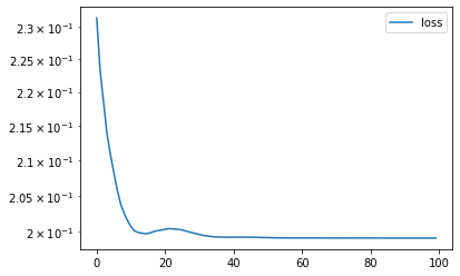
model = FourDimensionalOptimizer(average_roll=4.5)probabilities = model.optimize(iterations=100)total_probability =sum(probabilities)average_roll =sum( value * probabilityfor value, probability inenumerate(probabilities, start=1))print(f"Probabilities sum to: {total_probability:0.5f}")print(f"Average roll is: {average_roll:0.5f}")probabilities
        loss        p1       p2        p3        p4        p5        p6
91  0.199173  0.054391  0.07858  0.114577  0.165202  0.239592  0.347659
Probabilities sum to: 1.00000
Average roll is: 4.50000
model = FourDimensionalOptimizer( average_roll=3.5, initial_values=[1/6, 1/6, 1/6+0.1, 1/6-0.1])probabilities = model.optimize(iterations=100)total_probability =sum(probabilities)average_roll =sum( value * probabilityfor value, probability inenumerate(probabilities, start=1))print(f"Probabilities sum to: {total_probability:0.5f}")print(f"Average roll is: {average_roll:0.5f}")probabilities
        loss        p1        p2        p3       p4        p5        p6
99  0.166667  0.166787  0.166698  0.166547  0.16665  0.166334  0.166985
Probabilities sum to: 1.00000
Average roll is: 3.50000
This approach works much faster and we can see that it works for different roll averages too. It also produces values that are far more accurate.
1
2
3
4
5
6
model
0.054391
0.07858
0.114577
0.165202
0.239592
0.347659
correct
0.054
0.079
0.114
0.165
0.24
0.347
Looking at these the model is only out on \(p_3\) and \(p_6\) by 0.001 and that is due to rounding. This looks really solid.
TED Talk
This puzzle was set by a colleague and naturally he has his own solution. The solution he used allowed the model to optimize freely through the space and then maps the points back to the correct surface. I mentioned how I had found it hard to reason through the construction of the smaller space and he wrote this to me:
This is one of those rare cases where having a lot of mathematical training actually accomplishes something.Your approach of encoding the constraints into the objective function doesn’t have any major drawbacks that I can think of, except that it might be challenging to generalize it to nonlinear constraints - e.g. if the constraint is \(x^2 + y^2 = 1\) then you have to handle both the cases \(y = \sqrt{1 - x^2}\) and \(y = -\sqrt{1 - x^2}\).
Here’s how I thought through the projection approach (and again, there’s an element of training here - constructing projection maps is like what you do for breakfast every morning in functional analysis). First, we can express the constraint as \(Ax = b\). It is always easier to start equations of the form \(Ax = 0\) and then translate everything back, so we’ll start with that. Let’s pretend we’re working in 3 dimensions for a moment, and your equation looks like \(ax + by + cz = 0\). A good first step to constructing any matrix is to start with a nice coordinate system: we want coordinates \((u, v, w)\) with the properties that:
\(u\) and \(v\) lie in the plane
\(|u| = |v| = |w|\) (unit vectors)
dot products are all zero: \(\langle u,v \rangle = 0\), \(\langle u,w \rangle = 0\), \(\langle v,w \rangle = 0\)
This is called an “orthonormal basis” - the trick is starting with an orthonormal basis for the plane - in this case \(u\) and \(v\) - and extending it to the whole space. If you have such a thing, then the projection map is easy to construct: you just take dot products against \(u\) and \(v\): \(Px := \langle x,u \rangle u + \langle x,v \rangle v\). This lies in the plane because it is a linear combination of \(u\) and \(v\), and \(x - Px = \langle x,w \rangle w\) which is orthogonal to the plane. So the question is: “how do we come up with an orthonormal basis for a plane and extend it to the whole space?”. The answer is called the “Gram-Schmidt algorithm”, and it works like this:
Start with ANY basis \(b_1\), \(b_2\), \(b_3\) such that \(b_1\) and \(b_2\) are in the plane (just by solving the equation \(Ax = 0\)). Then iteratively build it up into an orthonormal basis by projecting:
\[
\begin{aligned}
u &= \frac{b1}{|b1|} \\
v &= b2 - proj(b2 -> u) = b2 - \langle b2, u \rangle u \\
v &= \frac{v}{|v|} \\
w &= b3 - proj(b3 -> u, v) = \dots \\
w &= \frac{w}{|w|} \\
\end{aligned}
\]
Now obviously I didn’t compute all that stuff in my solution, and the reason is that the other part of my training taught me that it is more numerically efficient to encode all of this algebra into matrix factorizations. So i went back and googled “which matrix factorizations use the gram-schmidt algorithm” and then pieced together the rest. Thank you for attending my ted talk.