Distillation is the process of training a small model on a task with the help of a larger, trained, model. The small model is referred to as the student and the large model is the teacher. Teaching the student involves the regular process of measuring accuracy and teaching the student to match the distribution of predictions from the teacher. Matching the distribution shows the student what other classes are similar to the correct class, and guides it to the correct weights in a more holistic way.
The teacher is large and well trained and that means that the teacher predicts the correct class very strongly. For the teacher to add value to the training we must alter this output to show the class distribution more. The way we do that is to alter the outputs, boosting the low probability classes and reducing the high probability class(es). Probability alteration is controlled using a parameter called temperature.
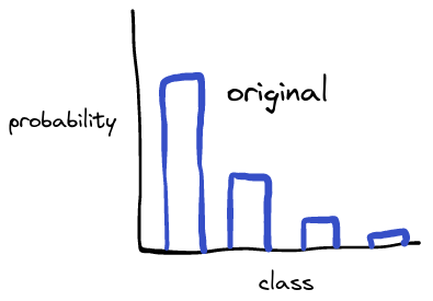
When trying out distillation I was concerned that the temperature parameter was not shaping the teacher output in an appropriate way. The teacher starts by strongly predicting a single class and the remaining probability is distributed between the other classes:
original output
The student is already being trained to correctly predict the class, the teacher is used to show appropriate decision boundaries. This means that the probability of the incorrect classes is what matters. Since the teacher strongly predicts the correct class, the influence of the incorrect classes is low.
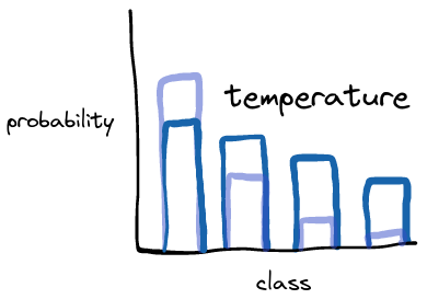
Temperature takes probability from the most confident class and reassigns it to the others:
temperature output
However the reassignment increases the probability of all of the classes together, meaning that the lowest probability classes get a significant boost.
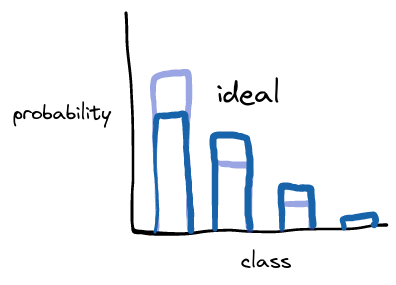
I think that it would be better if the probability was reassigned more to the more confident classes, and less to the less confident ones:
The new algorithm should retain the relative difference between classes. Since probability is being taken from the most confident class and reassigned to the other classes, the relative difference between the most confident class and other classes will change.
The new algorithm should reduce the top class and reassign the probability to the other classes. It should not alter the order of the classes, so there is no parameter value which will boost the second highest class above the highest class.
It should have the same value range as the original temperature, being one to infinity.
Retain Relative Difference
We can move probability while retaining relative difference by increasing the classes according to their existing probability. An example will show this more easily.
Given the probabilities \([0.5, 0.25, 0.15, 0.1]\), we want to reassign \(0.1\) of probability. We can calculate the ratio of each subsequent class by taking \(\text{ratio}_n = \frac{P_n}{\sum_{i=2}^{4} P_i}\). Multiplying the reassigned probability by this ratio will then produce the per-class increase.
For this example there is a ratio of \([0.5, 0.3, 0.2]\), meaning that the probabilities become \([0.4, 0.3, 0.18, 0.12]\).
We can then establish that the relative difference remains the same by taking the ratio of each number with it’s subsequent number:
Only one class gets a reduced probability - the most confident class. The probability that is reassigned from that is spread to the other classes according to the ratio, as described previously. This means that we can predict the point where the most confident class would swap places with the second most confident class:
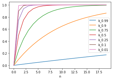
To have a range that extends to infinity with a finite change I want an asymptotic progression. It’s easy to come up with one, because I want the infinity point to be the change that makes the most confident class equal to the second most confident. That would be the full \(P_{change}\) from above.
This can be produced with \(1 - k^{n}\) where \(0 < k < 1\) and \(n\) is the new temperature parameter. We can see a few graphs of this:
Code
from typing import Dict, Unionimport pandas as pddef row(n: int) -> Dict[str, Union[float, int]]: values = {"n": n}for k in [0.99, 0.9, 0.75, 0.5, 0.25, 0.1, 0.01]: values[f"k_{k}"] = change(k=k, n=n)return valuesdef change(k: float, n: int) ->float:return1- k**n( pd.DataFrame([ row(n=n) for n inrange(20) ]) .set_index("n") .plot()) ;None
Looking at this I think that \(k = 0.9\) looks good as it changes significantly over the range without fully saturating.
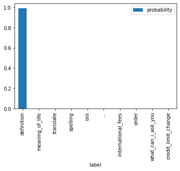
import pandas as pddf = top_and_bottom("what is the definiton of auspicious", tokenizer=tokenizer, model=model, temperature=1, k=0.5,)df.plot(x="label", y="probability", kind="bar")df.iloc[[0,1,9]]
label
probability
0
definition
0.991237
1
meaning_of_life
0.000330
9
credit_limit_change
0.000011
Code
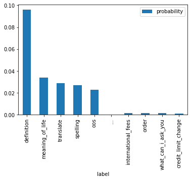
import pandas as pddf = top_and_bottom("what is the definiton of auspicious", tokenizer=tokenizer, model=model, temperature=5, k=0.5,)df.plot(x="label", y="probability", kind="bar")df.iloc[[0,1,9]]
label
probability
0
definition
0.096022
1
meaning_of_life
0.034091
9
credit_limit_change
0.001152
Code
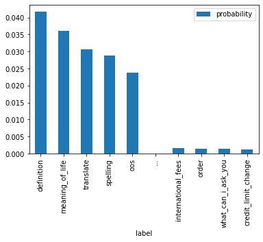
import pandas as pddf = top_and_bottom("what is the definiton of auspicious", tokenizer=tokenizer, model=model, temperature=19, k=0.75,)df.plot(x="label", y="probability", kind="bar")df.iloc[[0,1,9]]
label
probability
0
definition
0.041725
1
meaning_of_life
0.036138
9
credit_limit_change
0.001221
Code
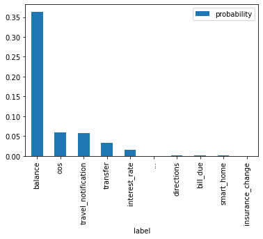
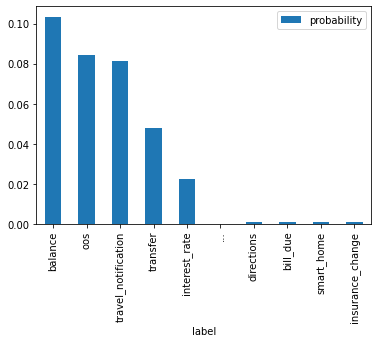
import pandas as pddf = top_and_bottom("Call me Ishmael. ""Some years ago, never mind how long precisely, ""having little or no money in my purse, ""and nothing particular to interest me on shore, ""I thought I would sail about a little and see the watery part of the world", tokenizer=tokenizer, model=model, temperature=1, k=0.5,)df.plot(x="label", y="probability", kind="bar")df.iloc[[0,1,9]]
label
probability
0
balance
0.363756
1
oos
0.059927
9
insurance_change
0.000506
Code
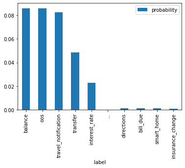
import pandas as pddf = top_and_bottom("Call me Ishmael. ""Some years ago, never mind how long precisely, ""having little or no money in my purse, ""and nothing particular to interest me on shore, ""I thought I would sail about a little and see the watery part of the world", tokenizer=tokenizer, model=model, temperature=5, k=0.5,)df.plot(x="label", y="probability", kind="bar")df.iloc[[0,1,9]]
label
probability
0
balance
0.103436
1
oos
0.084447
9
insurance_change
0.000713
Code
import pandas as pddf = top_and_bottom("Call me Ishmael. ""Some years ago, never mind how long precisely, ""having little or no money in my purse, ""and nothing particular to interest me on shore, ""I thought I would sail about a little and see the watery part of the world", tokenizer=tokenizer, model=model, temperature=19, k=0.5,)df.plot(x="label", y="probability", kind="bar")df.iloc[[0,1,9]]
label
probability
0
balance
0.086083
1
oos
0.086081
9
insurance_change
0.000727
Making it Batchwise
To apply this to distillation I need to make this work with batches instead of single elements. Since we have a working single row version it’s possible to use that to validate a simple batchwise version.
Now that we have a working batchwise version it can be used to validate a better version. When writing this my main concerns are to only perform batchwise operations. This takes advantage of the parallel performance that GPUs offer. The simple version iterates over the rows which performs very poorly on CUDA.
Code
def scale_batch( logits: torch.Tensor, temperature: float, k: float,) -> torch.Tensor: batch_size, output_size = logits.shape logits = logits.softmax(dim=1) logit_indices = logits.argsort(dim=1, descending=True)# when selecting multiple unaligned indices from a 2d tensor you can pass two lists# they are joined by index to determine the value to select:## t = torch.tensor(range(9)).reshape(3, 3)# >>> tensor([[0, 1, 2],# >>> [3, 4, 5],# >>> [6, 7, 8]])## t[[0, 1], [2, 0]]# >>> tensor([2, 3])## You can see that this has selected indices (0,2)=2 and (1,0)=3 rather than (0,1)=1 and (2,0)=6# This can be extended to select multi dimensionally:## t[[[0], [1]], [[2], [0]]]# >>> tensor([[2],# >>> [3]])## The shape of the output is the same as the shape of the index lookup# the single index is used when selecting a single index per batch single_index = torch.tensor(range(batch_size), device=logits.device)# the remaining index is used when selecting one less than all indices per batch rest_index = single_index[:, None].broadcast_to(batch_size, output_size -1)# these all have shape [batch_size, 1] top_probability = logits[single_index, logit_indices[:, 0]][:, None] remaining_probability =1- top_probability second_probability = logits[single_index, logit_indices[:, 1]][:, None] top_probability_change = (top_probability - second_probability) top_probability_change /=1+ (second_probability / remaining_probability) top_probability_change *=1- k ** (temperature -1)# this has a shape [batch_size, output_size-1] rest_probability = logits[rest_index, logit_indices[:, 1:]] rest_probability_change = top_probability_change * rest_probability / remaining_probability# if these changes are applied directly to logits then it breaks back propagation# generating an offset tensor that can be added to logits works fine offset = torch.zeros_like(logits) offset[single_index, logit_indices[:, 0]] =-top_probability_change[:, 0] offset[rest_index, logit_indices[:, 1:]] = rest_probability_changereturn logits + offset
Nice. I’m particularly pleased that the batchwise operations have perfectly duplicated the original. All of this is running on CPU so that is to be expected - on CUDA there is a chance of more change (especially if I turned on inference mode or amp).
Testing It
To establish if the new approach is better than the old I need to compare them. The new temperature parameter does not have the same scaling factor as the old one. If the same settings were used for the new approach and the old one there is no reason to believe they would both train well.
In the distillation workshop they had performed a parameter search to find appropriate settings. If I do the same for the two approaches then I can compare them.
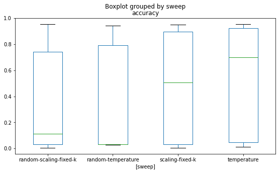
WandB can perform a bayesian search across continuous hyperparameters. This should have a reasonable chance at finding good parameters to use for the task. If I run this for both approaches then an approximate maximum accuracy can be achieved, which can then be compared.
It’s also possible to run a random sweep across the hyperparameters. This will show how well a random run would do. An approach that has a good average run could be used to try out distillation without requiring an expensive hyperparameter search.
The code below uses the WandB API to retrieve the run results.
You can see that the highest overall accuracy was achieved by the baesian search over the temperature hyperparameters. The maximum accuracy is very close with all approaches, but the higher average for the baesian temperature search suggests that it is a more predictable hyperparameter space.
The random searches show that the scaling approach is more likely to perform better with a random set of hyperparameters, however the average accuracy is still very poor (at about 0.1).
So the new approach that I have proposed is worse than the existing temperature approach. It also takes longer to compute.
Code and Runs
You can see the code here: https://gitlab.com/matthewfranglen/distillation-temperature
You can see the runs here: https://wandb.ai/matthewfranglen/distillation-temperature