Matthew’s Blog - Cross Language Prompt Internalization

I have calculated features using the XLM-RoBERTa base model for different links on wikipedia. If the student model is to be used for word sense induction then these features should cluster. A lack of clustering would show that this approach is not viable.

If clustering is viable the next step would be to work out an efficient way to test containment, as well as calculating an approximate smallest number of features required. The wikipedia processing was only 2% completed and I estimated it as taking 20 days so a way to reduce the work required would be great.

Load Features

The features have been written to a set of files, each of which contains 1,000 articles. Each article has an average of 30 links in it. Only 201 files were processed however that does give us slightly over 6 million features.

These features are not evenly distributed among the different articles so some of them will have a lot of features and some will have very few or none.

Code

from pathlib import Path
import pandas as pd

DATA_FOLDER = Path("/data/prompt-internalization/multilingual/wikipedia/enwiki/20220701/")

synonyms_df = pd.read_parquet(DATA_FOLDER / "synonyms.gz.parquet")
features_df = pd.concat([
    pd.read_parquet(file)
    for file in sorted((DATA_FOLDER / "features").glob("*.gz.parquet"))
])

Code

top_10_features = features_df.target.value_counts()[:10].index
top_10_features

Index(['united states', 'world war ii', 'new york city', 'france', 'england',
       'democratic party (united states)', 'united kingdom', 'london', 'india',
       'world war i'],
      dtype='object')

Code

top_10_rows = features_df[features_df.target.isin(top_10_features)]
top_10_rows = top_10_rows.copy()
top_10_rows["target"] = top_10_rows.target.astype("category")
top_10_rows = top_10_rows.reset_index(drop=True)
top_10_rows

	target	probability	index
0	france	[0.67140967, 0.21350534, 0.032488544, 0.031876...	[74831, 6557, 90788, 119862, 83658, 16843, 825...
1	united states	[0.6089455, 0.16102183, 0.053454213, 0.0463878...	[74831, 90788, 119862, 6557, 79200, 22836, 596...
2	world war ii	[0.20548585, 0.07137032, 0.066305555, 0.059100...	[48962, 42552, 72944, 65786, 5550, 60457, 7064...
3	france	[0.91993374, 0.043690596, 0.0077915695, 0.0053...	[74831, 6557, 83658, 90788, 119862, 16843, 228...
4	united states	[0.62910575, 0.114415355, 0.045016088, 0.01939...	[74831, 90788, 6557, 22836, 98148, 83658, 1198...
...	...	...	...
39958	new york city	[0.6512393, 0.1441473, 0.04517786, 0.028335713...	[90788, 74831, 6406, 79200, 6557, 16843, 49990...
39959	united states	[0.63683414, 0.089536354, 0.066114485, 0.03989...	[74831, 119862, 90788, 6557, 22836, 60457, 836...
39960	united states	[0.58584386, 0.1483111, 0.12411963, 0.02704905...	[74831, 90788, 6557, 119862, 82581, 22836, 168...
39961	new york city	[0.71458614, 0.06404259, 0.053600095, 0.039861...	[90788, 74831, 79200, 6406, 16843, 49990, 9814...
39962	england	[0.86271405, 0.06343852, 0.024254996, 0.014000...	[74831, 6557, 90788, 83658, 119862, 82581, 168...

39963 rows × 3 columns

We have almost 40,000 features for the top 10 articles. These articles are nice as they form into several distinct themes so we should expect articles like united states and england to be near to each other and united states and democratic party (united states) to be separated.

To be able to work with this I need to create a matrix that has the approximation of what the model produced. Each feature is the top 100 tokens split between the token index and probability. This matrix will be large though - the model has a vocabulary of 250,002 tokens, which will cause memory issues. Finding a smaller matrix that covers all the tokens that are non-zero would be good.

Code

import pandas as pd
import numpy as np

def to_probability_matrix(df: pd.DataFrame) -> np.array:
    unique_tokens = sorted(df["index"].explode().unique())
    token_map = {
        token_index: index
        for index, token_index in enumerate(unique_tokens)
    }
    rows = len(df)
    token_count = len(unique_tokens)

    def map_tokens(tokens: list[int]) -> list[int]:
        return list(map(token_map.get, tokens))
        
    token_index = np.array(df["index"].apply(map_tokens).tolist())
    probability = np.zeros((rows, token_count))
    probability.flat[
        token_index + (token_count * np.arange(rows)[:, None])
    ] = np.array(df.probability.tolist())

    return probability

Code

%%time

probability = to_probability_matrix(top_10_rows)

sums = probability.sum(axis=1)
print(sums.min(), sums.max(), sums.mean())
del sums
print(probability.shape)
print()

0.9999997086397343 1.0000002902579581 1.0000000003762612
(39963, 2192)

CPU times: user 923 ms, sys: 148 ms, total: 1.07 s
Wall time: 1.07 s

There are 10 separate articles and 100 tokens per link. If each article was always described in an identical way, and every different article was completely different, there would be 1,000 distinct tokens. We can see that there are 2,192 distinct tokens so this ideal state has not been achieved.

It should be possible to review how well the tokens overlap between the different labels.

Code

import pandas as pd

def get_iou_crosstab(df: pd.DataFrame) -> pd.DataFrame:
    labels = sorted(df.target.unique())
    df = df[["target", "index"]]
    df = df.explode("index")
    df = df.groupby("target").agg(set)

    intersection = {
        (left, right): len(df.loc[left][0] & df.loc[right][0])
        for left in labels
        for right in labels
    }
    union = {
        (left, right): len(df.loc[left][0] | df.loc[right][0])
        for left in labels
        for right in labels
    }
    return pd.DataFrame([
        {other: intersection[(label, other)] / union[(label, other)] for other in labels}
        for label in labels
    ], index=labels)

Code

iou_crosstab = get_iou_crosstab(top_10_rows)
iou_crosstab.style.highlight_quantile(q_left=0.5, axis=None, color='lightgreen')

	democratic party (united states)	england	france	india	london	new york city	united kingdom	united states	world war i	world war ii
democratic party (united states)	1.000000	0.334888	0.308453	0.354062	0.273659	0.320273	0.355752	0.346124	0.311338	0.271583
england	0.334888	1.000000	0.613659	0.608515	0.573287	0.511668	0.598338	0.537795	0.355219	0.306073
france	0.308453	0.613659	1.000000	0.592105	0.459889	0.441463	0.568365	0.489827	0.314562	0.276911
india	0.354062	0.608515	0.592105	1.000000	0.477408	0.481350	0.589595	0.531915	0.360320	0.304940
london	0.273659	0.573287	0.459889	0.477408	1.000000	0.598842	0.475347	0.462697	0.337808	0.280827
new york city	0.320273	0.511668	0.441463	0.481350	0.598842	1.000000	0.513912	0.490647	0.414894	0.339520
united kingdom	0.355752	0.598338	0.568365	0.589595	0.475347	0.513912	1.000000	0.589783	0.404762	0.350670
united states	0.346124	0.537795	0.489827	0.531915	0.462697	0.490647	0.589783	1.000000	0.359353	0.299329
world war i	0.311338	0.355219	0.314562	0.360320	0.337808	0.414894	0.404762	0.359353	1.000000	0.640577
world war ii	0.271583	0.306073	0.276911	0.304940	0.280827	0.339520	0.350670	0.299329	0.640577	1.000000

This crosstab is pretty encouraging. With the threshold of 0.5 it shows that:

the world war articles overlap only with each other
the political party doesn’t overlap with anything else
most of the countries overlap with each other and the cities

This is a really rough way to cluster this data. Let’s see the results of a more structured analysis.

2d Projection

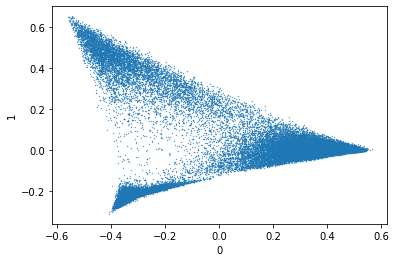
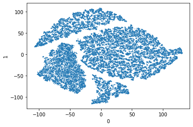
The first thing is to try out projecting this data into 2 dimensions so we can visualize it. I’m going to use my two favourite approaches of PCA and T-SNE.

Code

from sklearn.decomposition import PCA

pca_output = PCA(
    n_components=2,
    random_state=0,
).fit_transform(probability)
pca_df = pd.DataFrame(pca_output)
pca_df["target"] = top_10_rows.target.values

pca_df.plot.scatter(x=0, y=1, s=0.1) ; None

Code

from sklearn.decomposition import PCA
from sklearn.manifold import TSNE
import numpy as np

n_components = 2

# doing this to avoid the warning about future T-SNE
tsne_init = (
    PCA(
        n_components=n_components,
        svd_solver="randomized",
        random_state=0,
    )
        .fit_transform(probability)
        .astype(np.float32, copy=False)
)

tsne_output = TSNE(
    n_components=n_components,
    learning_rate="auto",
    init=tsne_init,
).fit_transform(probability)
tsne_df = pd.DataFrame(tsne_output)
tsne_df["target"] = top_10_rows.target.values

tsne_df.plot.scatter(x=0, y=1, s=0.1) ; None

Here it looks like the data has become a triangle with PCA and four clearly separate islands with T-SNE. This is interesting as it shows both clear structure and a lower set of clusters compared to the number of labels (remember it’s the top 10 labels).

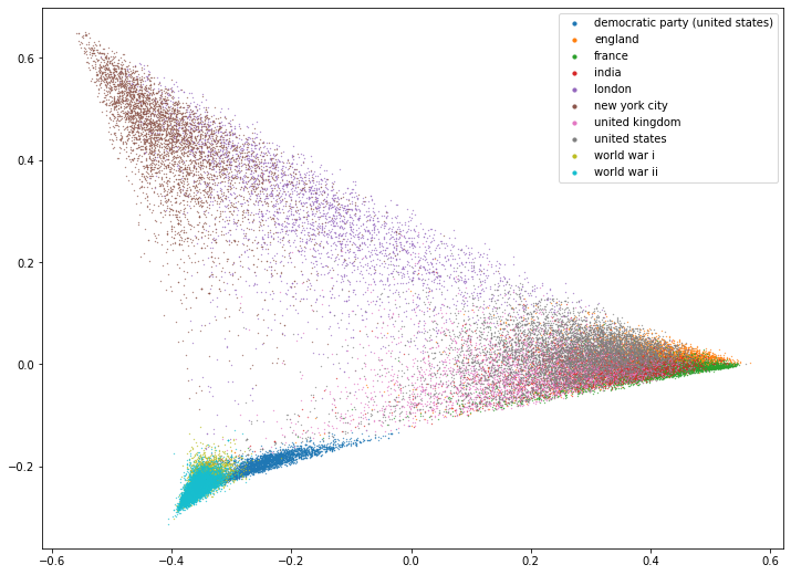
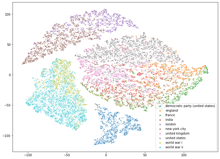
Let’s try coloring this data by the label.

Code

from typing import List, Optional
import matplotlib.pyplot as plt
import pandas as pd

def plot_2d(df: pd.DataFrame, targets: Optional[List[str]] = None) -> None:
    fig, ax = plt.subplots(figsize=(12, 9))

    for group_name, group_idx in df.groupby("target").groups.items():
        if targets and group_name not in targets:
            continue
        ax.scatter(
            *df.iloc[group_idx, [0, 1]].T.values,
            s=0.1,
            label=group_name
        )
    ax.legend(markerscale=10)

Code

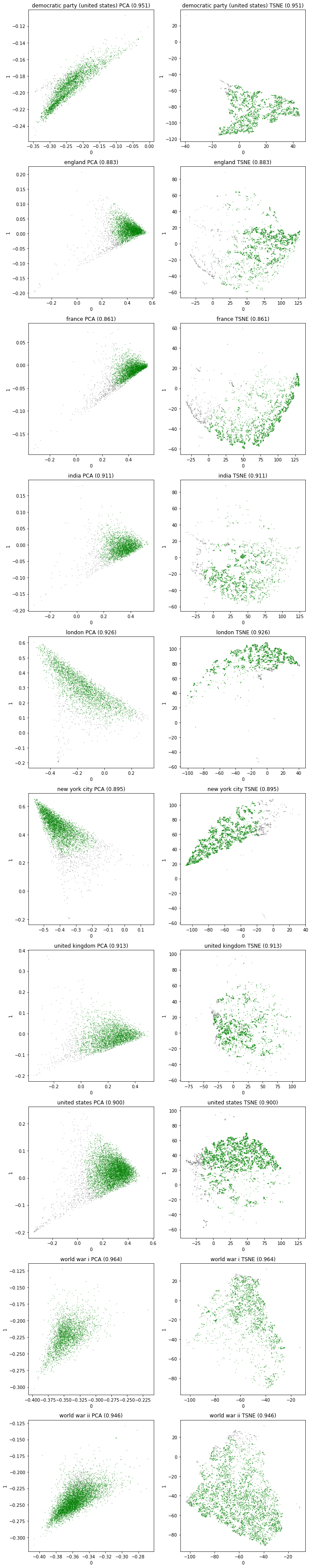
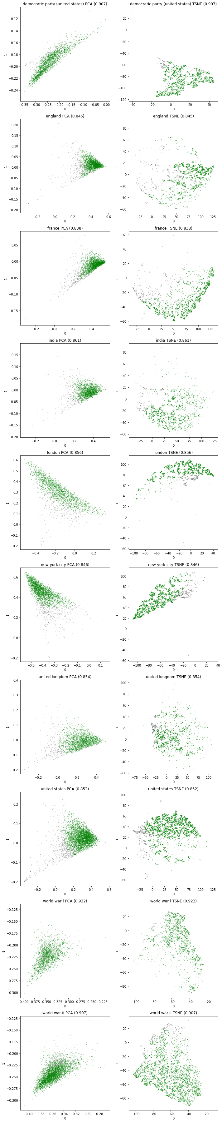
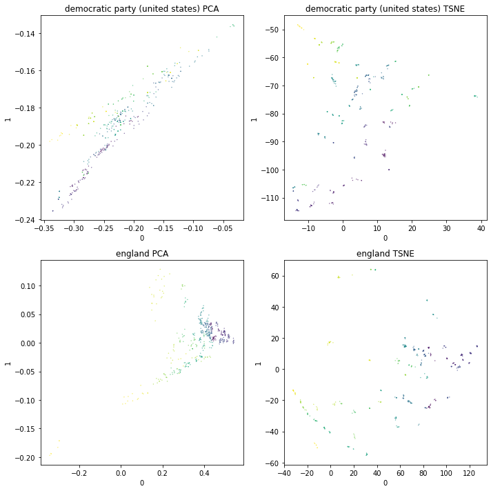
plot_2d(pca_df)

Code

plot_2d(tsne_df)

The clusters do have mostly consistent color. I’m pleased that the democratic party is a separate isolated cluster which has very little overlap with the other labels. The T-SNE projection suggests that there are four distinct clusters in this data, being:

The democratic party (bottom center)
The world wars (left)
London and New York (top)
The countries (right)

Which is encouraging as it suggests that the cities can be cleanly separated from the countries.

PCA looks like it extends in another dimension as the shape reminds me of an old origami fold that I was fond of:

I wonder if the labels separate more clearly in 3d.

3d Projection

PCA and T-SNE are not restricted to projecting to 2 dimensions. Given that the PCA projection in particular looks like it has a significant third dimension I’m interested in visualizing it.

Code

from sklearn.decomposition import PCA

pca = PCA(n_components=3, random_state=0)
pca.fit(probability.T)
pca_3d_df = pd.DataFrame(pca.components_.T)
pca_3d_df["target"] = top_10_rows["target"].values

Code

from sklearn.decomposition import PCA
from sklearn.manifold import TSNE
import numpy as np

n_components = 3

# doing this to avoid the warning about future T-SNE
tsne_init = (
    PCA(
        n_components=n_components,
        svd_solver="randomized",
        random_state=0,
    )
        .fit_transform(probability)
        .astype(np.float32, copy=False)
)

tsne_output = TSNE(
    n_components=n_components,
    learning_rate="auto",
    init=tsne_init,
).fit_transform(probability)
tsne_3d_df = pd.DataFrame(tsne_output)
tsne_3d_df["target"] = top_10_rows.target.values

Code

from typing import List, Optional
import matplotlib.pyplot as plt
from mpl_toolkits.mplot3d import Axes3D
import pandas as pd

def plot_3d(df: pd.DataFrame, targets: Optional[List[str]] = None) -> None:
    fig = plt.figure(figsize=(12, 9))
    ax = Axes3D(fig, auto_add_to_figure=False)
    fig.add_axes(ax)

    for group_name, group_idx in df.groupby("target").groups.items():
        if targets and group_name not in targets:
            continue
        ax.scatter(
            *df.iloc[group_idx, [0, 1, 2]].T.values,
            s=0.1,
            label=group_name
        )
    ax.legend(markerscale=10)

Code

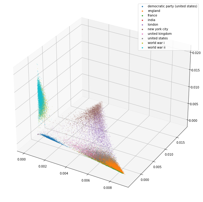
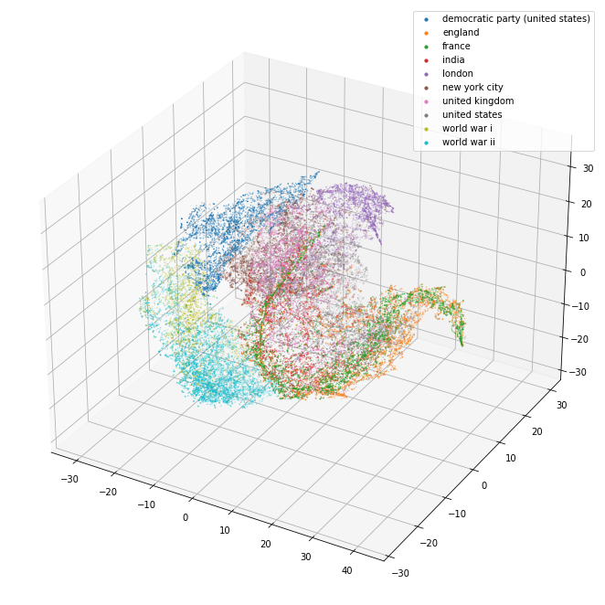
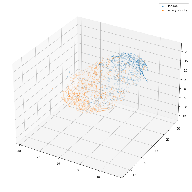
plot_3d(pca_3d_df)

Projecting this into 3d has shown something similar to the shape that I suspected. It’s almost a shame that I can’t rotate that projection a little to see it better. We can now try separating out the different labels into related groups to see if they are clustered near to each other.

Code

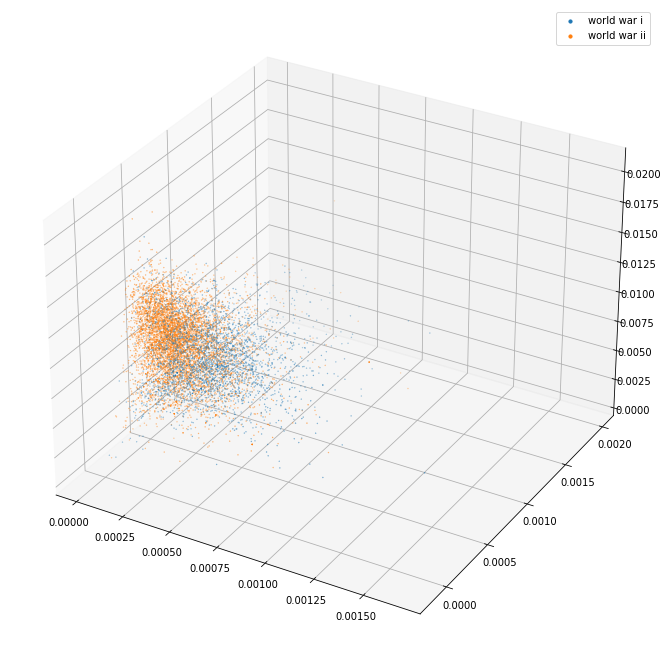
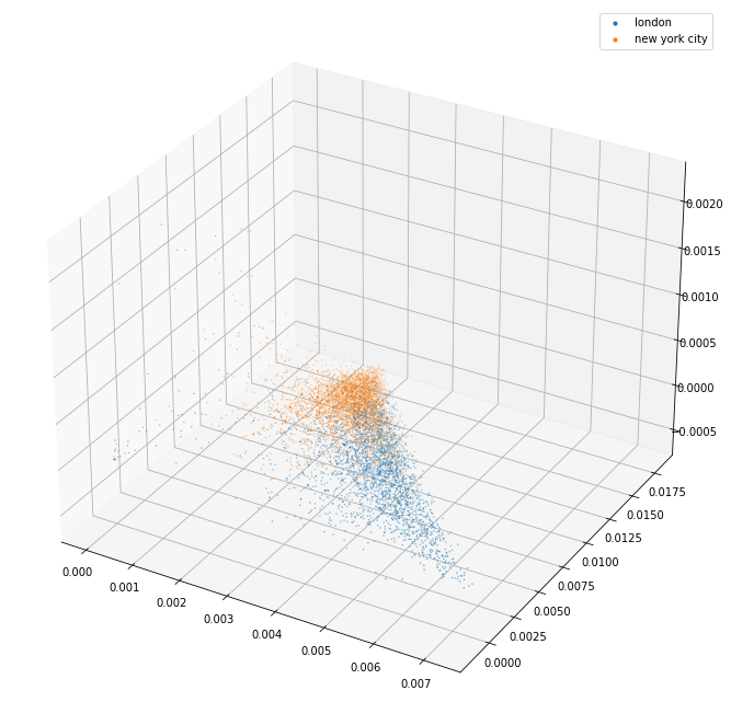
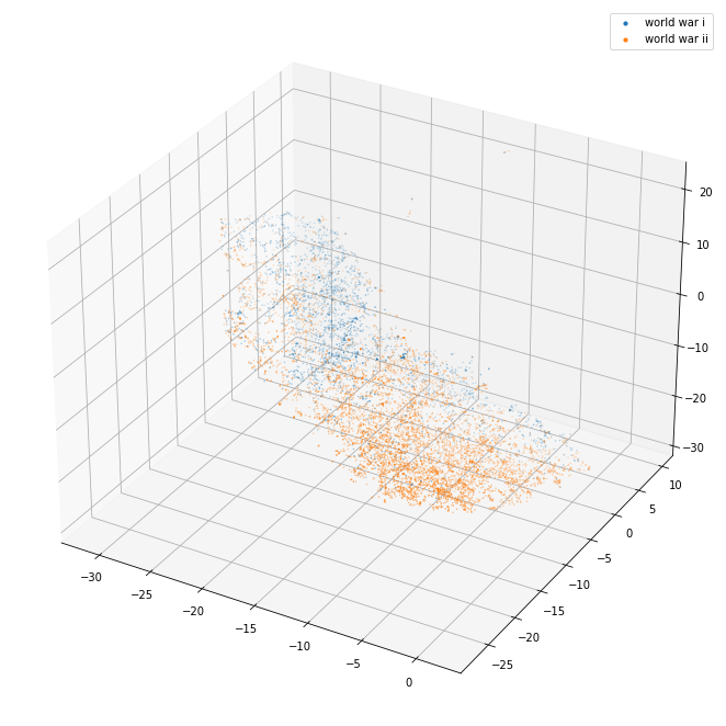
plot_3d(pca_3d_df, ["world war i", "world war ii"])

Code

plot_3d(pca_3d_df, ["united kingdom", "united states", "england", "france", "india"])

Code

plot_3d(pca_3d_df, ["london", "new york city"])

Code

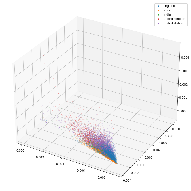
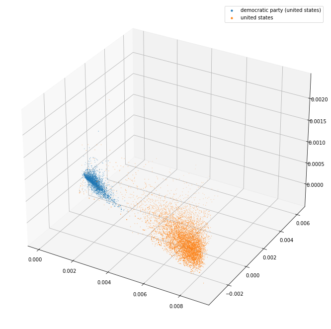
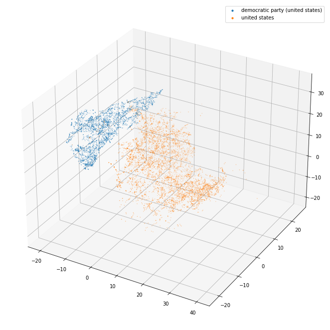
plot_3d(pca_3d_df, ["democratic party (united states)", "united states"])

The 3d projection helps a lot. I can see here that the separation between the separate kinds of things (political party/world war/city/country) seems pretty good. The countries in particular are blended together so it may well be that they are quite similar and that distinguishing them might be tricky.

We can repeat this with T-SNE, however that already looks like a complex structure so I am not sure how much this will help.

Code

plot_3d(tsne_3d_df)

Code

plot_3d(tsne_3d_df, ["world war i", "world war ii"])

Code

plot_3d(tsne_3d_df, ["united kingdom", "united states", "england", "france", "india"])

Code

plot_3d(tsne_3d_df, ["london", "new york city"])

Code

plot_3d(tsne_3d_df, ["democratic party (united states)", "united states"])

The T-SNE projection might look pretty but the clarity of the separate clusters is somewhat lacking. I’m satisfied with the PCA projection results though.

Clustering New Points

Having these clusters is nice. What I need is to be able to define these clusters in a way where I can test new points to see if they lie within.

Given that the labels do not form nice spherical shapes I do not think that KMeans would be appropriate. Something that can track the shape more accurately could be better.

I like using (H)DBSCAN as it can track arbitrary shapes. Working with that over a large number of labels could be tricky so I may need to optimize this in future.

The biggest problem with using DBSCAN is coming up with appropriate values for eps and min_samples.

Code

probability_df = pd.DataFrame(
    {"probability": list(probability)},
    index=top_10_rows.index
)
probability_df["target"] = top_10_rows.target.values

Code

from sklearn.neighbors import NearestNeighbors
from sklearn.cluster import DBSCAN
import numpy as np

def dbscan_label(df: pd.DataFrame, min_samples_ratio: float) -> (list[int], int):
    dbscan, most_common_label = run_dbscan(
        df=df,
        min_samples_ratio=min_samples_ratio,
    )
    return dbscan.labels_, most_common_label

def run_dbscan(df: pd.DataFrame, min_samples_ratio: float) -> (DBSCAN, int):
    probability = np.array(df.probability.tolist())
    min_samples = max(1, int(len(df) * min_samples_ratio))

    neighbors = NearestNeighbors(n_neighbors=min_samples)
    neighbors.fit(probability)

    neighbor_distance, _ = neighbors.kneighbors(X=probability, n_neighbors=min_samples)
    # 75% quantile distance that encompasses all min_samples points
    median_eps = np.quantile(neighbor_distance[:, -1], 0.75)

    dbscan = DBSCAN(eps=median_eps, min_samples=min_samples)
    dbscan.fit(probability)

    labels = pd.Series(dbscan.labels_)
    labels = labels[labels != -1]
    most_common_label = labels.value_counts().index[0]

    return dbscan, most_common_label

Code

import matplotlib.pyplot as plt
from sklearn.cluster import DBSCAN
import pandas as pd


def plot_dbscan_by_label(
    df: pd.DataFrame,
    pca_df: pd.DataFrame,
    tsne_df: pd.DataFrame,
    min_samples_ratio: float,
) -> None:
    labels = sorted(df.target.unique())
    rows = len(labels)

    fig, axes = plt.subplots(rows,2, figsize=(10,5*rows))
    for label, (ax_pca, ax_tsne) in zip(labels, axes):
        label_df = df[probability_df.target == label].copy()
        cluster_labels, primary_cluster = dbscan_label(
            df=label_df,
            min_samples_ratio=min_samples_ratio,
        )
        ratio = (np.array(cluster_labels) == primary_cluster).sum() / len(label_df)

        probability_cluster_df = pca_df[pca_df.target == label].copy()
        probability_cluster_df["color"] = cluster_labels
        probability_cluster_df["color"] = probability_cluster_df.color == primary_cluster
        probability_cluster_df["color"] = probability_cluster_df["color"].map({True: "green", False: "grey"})
        probability_cluster_df.plot.scatter(
            x=0,
            y=1,
            c="color",
            s=0.1,
            ax=ax_pca,
            legend=False,
            title=f"{label} PCA ({ratio:0.3f})",
            colorbar=False,
            xlabel=None,
            ylabel=None,
        )

        probability_cluster_df = tsne_df[tsne_df.target == label].copy()
        probability_cluster_df["color"] = cluster_labels
        probability_cluster_df["color"] = probability_cluster_df.color == primary_cluster
        probability_cluster_df["color"] = probability_cluster_df["color"].map({True: "green", False: "grey"})
        probability_cluster_df.plot.scatter(
            x=0,
            y=1,
            c="color",
            s=0.1,
            colormap="viridis",
            ax=ax_tsne,
            legend=False,
            title=f"{label} TSNE ({ratio:0.3f})",
            colorbar=False,
            xlabel=None,
            ylabel=None,
        )

    plt.tight_layout()  # Optional ... often improves the layout

Code

plot_dbscan_by_label(
    df=probability_df,
    pca_df=pca_df,
    tsne_df=tsne_df,
    min_samples_ratio=0.1
)

Code

plot_dbscan_by_label(df=probability_df, pca_df=pca_df, tsne_df=tsne_df, min_samples_ratio=0.01)

This doesn’t seem terrible? When considering these it is more significant to work out what the labelling would be for the wrong classes. As I see it DBSCAN is a very off/on classification where I may need a more continuous metric to allow for dispute resolution.

Code

def dbscan_predict(model: DBSCAN, points: np.array) -> np.array:
    point_count = points.shape[0]
    result = np.ones(shape=point_count, dtype=int) * -1
    for i in range(point_count):
        difference = model.components_ - points[i, :]
        distance = np.linalg.norm(difference, axis=1)
        closest_idx = np.argmin(distance)
        if distance[closest_idx] < model.eps:
            result[i] = model.labels_[model.core_sample_indices_[closest_idx]]
    return result

Code

import matplotlib.pyplot as plt
from sklearn.cluster import DBSCAN
import pandas as pd
from tqdm.auto import tqdm

def dbscan_iou_crosstab(df: pd.DataFrame, min_samples_ratio: float) -> pd.DataFrame:
    labels = sorted(df.target.unique())
    rows = len(labels)
    probability = np.array(df.probability.tolist())

    classifiers: dict[str, (DBSCAN, int)] = {
        label: run_dbscan(
            df=df[df.target == label],
            min_samples_ratio=min_samples_ratio,
        )
        for label in labels
    }
    
    def get_predictions(model: DBSCAN, index: int) -> pd.Series:
        cluster_indices = dbscan_predict(model, probability)
        predictions = cluster_indices == index
        return (
            pd.DataFrame({"target": df.target, "label": predictions})
                .groupby("target")
                .agg(sum)
                .label
        )

    result = pd.DataFrame([
        get_predictions(*classifiers[label])
        for label in tqdm(labels)
    ], index=labels)
    rows_per_label = df.groupby("target").agg(len).probability
    return result.divide(rows_per_label, axis="columns")

Code

dbscan_crosstab_01 = dbscan_iou_crosstab(probability_df, min_samples_ratio=0.1)
dbscan_crosstab_01.style.highlight_between(left=0.1, axis=None, color='lightgreen')

target	democratic party (united states)	england	france	india	london	new york city	united kingdom	united states	world war i	world war ii
democratic party (united states)	0.950913	0.000000	0.000000	0.000000	0.000000	0.000000	0.000000	0.000000	0.000000	0.000000
england	0.000000	0.883395	0.820830	0.657761	0.000646	0.000000	0.315442	0.484727	0.000000	0.000000
france	0.000000	0.848814	0.860951	0.670612	0.000000	0.000000	0.241379	0.241993	0.000000	0.000000
india	0.000000	0.953701	0.929651	0.910720	0.001291	0.000000	0.595502	0.690540	0.000000	0.000000
london	0.000000	0.005716	0.000000	0.004058	0.926081	0.897688	0.039880	0.066578	0.000000	0.000000
new york city	0.000000	0.000000	0.000000	0.000000	0.358618	0.895171	0.000300	0.000000	0.000000	0.000000
united kingdom	0.000000	0.975707	0.964001	0.967535	0.057456	0.000000	0.913343	0.946916	0.000000	0.000000
united states	0.000000	0.937696	0.884858	0.876902	0.041963	0.000000	0.709145	0.900208	0.000000	0.000000
world war i	0.000000	0.000000	0.000000	0.000000	0.000000	0.000000	0.000300	0.000000	0.963760	0.933968
world war ii	0.000000	0.000000	0.000000	0.000000	0.000000	0.000000	0.000000	0.000000	0.840330	0.945915

Code

dbscan_crosstab_001 = dbscan_iou_crosstab(probability_df, min_samples_ratio=0.01)
dbscan_crosstab_001.style.highlight_between(left=0.1, axis=None, color='lightgreen')

target	democratic party (united states)	england	france	india	london	new york city	united kingdom	united states	world war i	world war ii
democratic party (united states)	0.906615	0.000000	0.000000	0.000000	0.000000	0.000000	0.000000	0.000000	0.000000	0.000000
england	0.000000	0.844813	0.805441	0.533311	0.000000	0.000000	0.165517	0.228944	0.000000	0.000000
france	0.000000	0.709060	0.837318	0.510991	0.000000	0.000000	0.088756	0.049822	0.000000	0.000000
india	0.000000	0.909403	0.897499	0.860670	0.000000	0.000000	0.354723	0.358986	0.000000	0.000000
london	0.000000	0.001715	0.000000	0.001691	0.856359	0.722820	0.010495	0.027432	0.000000	0.000000
new york city	0.000000	0.000000	0.000000	0.000000	0.344416	0.845502	0.000000	0.000000	0.000000	0.000000
united kingdom	0.000000	0.957702	0.944490	0.923909	0.023564	0.000000	0.851574	0.883452	0.000000	0.000000
united states	0.000000	0.903973	0.820280	0.778154	0.017753	0.000000	0.587406	0.851868	0.000000	0.000000
world war i	0.000000	0.000000	0.000000	0.000000	0.000000	0.000000	0.000300	0.000000	0.921780	0.808847
world war ii	0.000000	0.000000	0.000000	0.000000	0.000000	0.000000	0.000000	0.000000	0.753140	0.907491

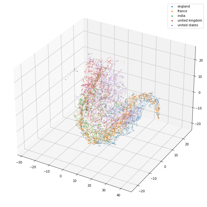
Using DBSCAN as the clustering shows much stronger performance. At this point the cities / countries are separated. Just from clustering this seems good enough as the actual text that was linked can be used as a signal to separate the intermingled cluster into the specific article.

Clustering with OPTIC

The sklearn documentation for DBSCAN also mentions OPTIC as an alternative which requires less configuration. Given that eps / max_samples are hard to calculate it might be worth trying.

Code

import matplotlib.pyplot as plt
from sklearn.cluster import OPTICS

# min_samples_ratio = 1/4 # 1_000 # 1_000 // 2**4
# eps = 1/2**3

labels = sorted(probability_df.target.unique())[:2]
rows = len(labels)

fig, axes = plt.subplots(rows,2, figsize=(10,5*rows))
for label, (ax_pca, ax_tsne) in zip(labels, axes):
    labelled_probability = probability_df[probability_df.target == label]
    # min_samples = int(len(labelled_probability) * min_samples_ratio)

    cluster_output = (
        OPTICS()
            .fit(np.array(labelled_probability.probability.tolist()))
    )

    probability_cluster_df = pca_df[pca_df.target == label].copy()
    probability_cluster_df["color"] = cluster_output.labels_
    probability_cluster_df = probability_cluster_df[probability_cluster_df.color != -1]
    probability_cluster_df.plot.scatter(
        x=0,
        y=1,
        c="color",
        s=0.1,
        colormap="viridis",
        ax=ax_pca,
        legend=False,
        title=f"{label} PCA",
        colorbar=False,
        xlabel=None,
        ylabel=None,
    )
    
    probability_cluster_df = tsne_df[tsne_df.target == label].copy()
    probability_cluster_df["color"] = cluster_output.labels_
    probability_cluster_df = probability_cluster_df[probability_cluster_df.color != -1]
    probability_cluster_df.plot.scatter(
        x=0,
        y=1,
        c="color",
        s=0.1,
        colormap="viridis",
        ax=ax_tsne,
        legend=False,
        title=f"{label} TSNE",
        colorbar=False,
        xlabel=None,
        ylabel=None,
    )

plt.tight_layout()  # Optional ... often improves the layout

/home/matthew/.cache/pypoetry/virtualenvs/blog-HrtMnrOS-py3.10/lib/python3.10/site-packages/sklearn/cluster/_optics.py:903: RuntimeWarning: divide by zero encountered in divide
  ratio = reachability_plot[:-1] / reachability_plot[1:]
/home/matthew/.cache/pypoetry/virtualenvs/blog-HrtMnrOS-py3.10/lib/python3.10/site-packages/sklearn/cluster/_optics.py:903: RuntimeWarning: divide by zero encountered in divide
  ratio = reachability_plot[:-1] / reachability_plot[1:]

This is incredibly slow to run and it smashes the data into tiny clusters. Given the lack of configuration it’s not really a viable system.