Cross Language Prompt Internalization - Wikipedia Synonym Clustering

In the previous post I looked into how the features from the model form into clusters and if it was viable to use them to perform Word Sense Induction. I found that related clusters overlap heavily and that a reliable resolution for a given word is not possible by only using cluster containment.

In this post I am going to investigate combining the model features with the list of synonyms for a given article. A synonym in this is the text that is linked to the article and as such is considered a valid term with which to reference the article.

To perform this evaluation I need more structured data as I must be able to combine both the specific term in the text with the model output. I will be evaluating both the prompted teacher, as well as the unprompted student. If this goes well then I hope I can use it to provide a more reliable metric for student evaluation.

Load Data

Loading the features and synonyms can be done quite easily

Code

from pathlib import Path
import pandas as pd

DATA_FOLDER = Path("/data/prompt-internalization/multilingual/wikipedia/enwiki/20220701/")

synonyms_df = pd.read_parquet(DATA_FOLDER / "synonyms.gz.parquet")
features_df = pd.concat([
    pd.read_parquet(file)
    for file in sorted((DATA_FOLDER / "features").glob("*.gz.parquet"))
])

The features are still tricky. For each article there are a number of descriptions that the model has given based on links. These descriptions are the top 100 tokens that were predicted along with their probability. When taken as a group this describes an article space - a new point that is within that space may be from a word or phrase describing that article.

What I want there is to be able to assign a probability of being within the space to an arbitrary point. I’ve tried using DBSCAN for this, but it is too slow. Filtering only on the tokens that are used to describe the space at all is close, but it does not form a continuous space that would allow for discrimination.

I feel like a probability approach can work if the different dimensions of the feature are described. If we have the mean and standard deviation for each feature that is associated with an article then it should be possible to compute the probability that a point lies within that article space.

Code

articles = set(
    synonyms_df[synonyms_df.synonym == "target"]
        .sort_values(by="count", ascending=False)
        .target
        .unique()
)
target_df = features_df[features_df.target.isin(articles)]
target_df.target.value_counts()[:5]

target corporation         103
translation                 64
receptor (biochemistry)     48
target ship                 19
target australia            16
Name: target, dtype: int64

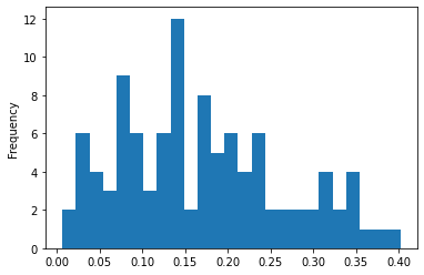
This is a reasonably ambiguous word that also has a meaning not described by the above articles (a desired goal). Ideally if given the “goal” sense of the word it would not disambiguate it as any of the above.

To achieve this I need a way to compute the probability that a given model output is within the word sense cluster.

Computing Word Sense Probability Cluster

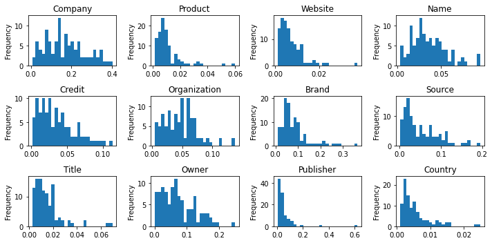
Given the target corporation features above it should be possible to define a cluster. If we take the different tokens that form the cluster we can plot the values that they take. Ideally this would form a normal distribution, which would then allow us to use the mean and standard deviation to calculate the probability that a point lies within the distribution.

Code

target_df[target_df.target == "target corporation"]["index"].explode().value_counts()

33734     103
73111     103
14737     103
15757     103
68021     103
         ... 
19055       1
91690       1
128896      1
49434       1
36293       1
Name: index, Length: 405, dtype: int64

Looking at the Token Distribution

We can check the distribution of the token values. Since we want to use a probability calculation that is based on a normal distribution it’s quite important that the tokens actually form a normal distribution.

Code

from typing import Callable
import pandas as pd
import numpy as np
from transformers import AutoTokenizer
import matplotlib.pyplot as plt

target_corporation_df = target_df[target_df.target == "target corporation"]

token_probability_df = pd.DataFrame(
    target_corporation_df.apply(
        lambda row: dict(zip(row["index"], row["probability"])),
        axis="columns"
    ).tolist()
)
tokens = target_corporation_df["index"].explode().value_counts().index

tokenizer = AutoTokenizer.from_pretrained("xlm-roberta-base")

rows = 12
fig, axes = plt.subplots(rows // 4, 4, figsize=(10,5))
for token, ax in zip(tokens, axes.flatten()):
    token_probability_df[token].plot.hist(bins=25, title=tokenizer.decode(token), ax=ax)
fig.tight_layout()

There are a couple of problems with this. First off, these are some very poor bell curves. The volume of data involved here is a bit of a problem so the curves might smooth if more was available. That’s quite a big assumption when some of these look more like a power law.

The second is that if these are bell curves then a lot of these are centered around zero. For example Publisher has the highest point at the zero+ bucket. It might be reasonable to assume that the zero point forms the center of the curve, but due to the mathematical preprocessing it is impossible to get negative values for a given token.

I’m also concerned about the effectiveness of comparisons involving this. For the comparison to be meaningful the softmax should be taken after the model output is restricted to the top 100 tokens. Once that has been done how do you compare a token index if it didn’t make the cut on one side?

Probability Calculation

I would like to calculate the combined probability:

\[ \prod_{i=0}^{100} P_i \]

This tends to suffer from underflow problems so the sum of the log probability is normally used:

\[ \sum_{i=0}^{100} \log(P_i) \]

The logarithm of zero is \(-\infty\), how could a sum be meaningful after that? How can I come up with a reasonable substitute for the probability of a token that falls out of the top 100?

If I ignore the token then the points that have a smaller token overlap actually get boosted as they have fewer terms in the sum. Would it be reasonable to take the final token probability as the probability of all unseen tokens?

Code

top_token_probabilities = token_probability_df[tokens[0]]
top_token_probabilities.plot.hist(bins=25)
top_token_probabilities.describe()

count    103.000000
mean       0.169728
std        0.094962
min        0.006392
25%        0.094385
50%        0.151124
75%        0.231087
max        0.401848
Name: 33734, dtype: float64

Code

from scipy.stats import norm

norm.pdf(
    [0, 0.15, 1],
    loc=top_token_probabilities.mean(),
    scale=top_token_probabilities.std(),
)

array([8.50509862e-01, 4.11137445e+00, 1.05671351e-16])

I find it strange that the probability function from scipy returns a value greater than one. It’s so strange that someone else asked about it on stack overflow.

I’m quite keen to be able to work with the concept of probability as it is easier for me to handle. Especially since the function above is capable of producing an infinite output.

We can try working with a permuted value where we calculate the continuous probability across a small area around the point.

Code

from scipy.stats import norm

np.sum(
    norm.cdf(
        np.array([0, 0.15, 1])[:, None] + np.array([-0.01, 0.01])[None, :],
        loc=top_token_probabilities.mean(),
        scale=top_token_probabilities.std(),
    ) * np.array([-1, 1])[None, :],
    axis=1
)

array([0.01707908, 0.08208231, 0.        ])

These values don’t seem terrible as the distribution is weighted towards the start with the mean of 0.16. A value of 1.0 would be almost 9 standard deviations away.

Testing Function Invocation

The norm functions can take arrays for the input, loc (mean) and scale (std). It would be good to understand how to use these correctly before proceeding.

I want to check that given a vector of values and a vector of mean/std I can calculate the probability in a single call instead of a call per value.

Code

values = np.random.normal(loc=0, scale=1, size=5)
mean = np.array([0., 0.2, 0.5, 1.0, -1.0])
std = np.array([1., 0.8, 0.5, 2.0, 0.1])

expected = np.array([
    norm.cdf(values[i], loc=mean[i], scale=std[i])
    for i in range(5)
])
actual = norm.cdf(
    values,
    loc=mean,
    scale=std,
)

(expected == actual).all()

True

This is good. It’s interesting to know that if the values is 2d then the comparison fails! (replace the assigment of values size with (5, 5) to see) We won’t be using that so no need to worry about it right now.

The next thing to check is the use of the permutation is consistent.

Code

values = np.random.normal(loc=0, scale=1, size=5)
mean = np.array([0., 0.2, 0.5, 1.0, -1.0])
std = np.array([1., 0.8, 0.5, 2.0, 0.1])

permutation = np.array([-0.01, 0.01])

expected = np.array([
    norm.cdf(values[i] + permutation, loc=mean[i], scale=std[i])
    for i in range(5)
])
actual = norm.cdf(
    values[:, None] + permutation[None, :],
    loc=mean[:, None],
    scale=std[:, None],
)

(expected == actual).all()

True

The final thing to check is that I can look up matching token indices in two arrays. When creating the description of a feature I will have a list of token indicies and an aligned list of probabilities.

I’m going to reduce the input features to the list of 100 before applying softmax to make it as similar as possible to the way the original features were extracted. This then requires aligning the input tokens with the tokens that the cluster has used.

I’ve found a stack overflow post about producing such alignment but it’s quite difficult to understand so I want to write a simple version and then test that the complex one is the same.

Code

import random

# This is the wikipedia article list of token indices and their values.
# There can be no repeated indices and they have to be sorted.
feature_indices = np.sort(
    np.array(random.sample(range(1_000), 400))
)
feature_values = np.random.normal(loc=0, scale=1, size=400)

# This is the current sentence features.
# Again, no repeating values, must be sorted.
point_indices = np.sort(
    np.array(random.sample(range(1_000), 100))
)
point_values = np.random.normal(loc=0, scale=1, size=100)

expected_p2f = np.array([
    (index == feature_indices).nonzero()[0][0]
    for index in point_indices
    if index in feature_indices
])

# If you look at the name it's point to feature
# but the argument to in1d is feature followed by point.
actual_p2f = np.where(np.in1d(feature_indices, point_indices))[0]

# the next thing is that these indices are only valid for points that HAVE a mapping.
# I'm happy to reduce the point values down like this because handling undescribed points is important.
# The feature index and values cannot be routinely mutated like this as that is the reference.
expected_point_indices = np.array([
    index
    for index in point_indices
    if index in feature_indices
])
# the in1d is reversed again! This time it is checking point in feature
actual_point_indices = point_indices[np.in1d(point_indices, feature_indices)]

assert (actual_point_indices == expected_point_indices).all()

# We can verify the direction by checking index values:
assert actual_point_indices[0] == feature_indices[actual_p2f[0]]

expected_f2p = np.array([
    (index == point_indices).nonzero()[0][0]
    for index in feature_indices
    if index in point_indices
])
actual_f2p = np.where(np.in1d(point_indices, feature_indices))[0]

(actual_p2f == expected_p2f).all(), (actual_f2p == expected_f2p).all()

(True, True)

That’s quite complex but I’m glad I did it. Writing this stuff out correctly is complex. As an engineer in a past life I want to write the efficient code first time heh.

Probability Comparison

Let’s see how the cumulative probabilities of the features for target corporation compare to those for translation. To work with this I need some actual model outputs as this will be comparing the model output to the features that most commonly describe the wikipedia article.

Code

from transformers import AutoTokenizer, AutoModelForMaskedLM

MODEL_NAME = "xlm-roberta-base"
model = AutoModelForMaskedLM.from_pretrained(MODEL_NAME)
model.eval()
tokenizer = AutoTokenizer.from_pretrained(MODEL_NAME)

Code

import torch
import numpy as np

@torch.inference_mode()
def get_prediction(
    text: str,
    noun: str,
    prompt: str = " Pet: Dog, Color: Yellow, Vehicle: Tractor, Fruit: Banana,<mask>: {}",
) -> np.array:
    input_ids = tokenizer(
        text.strip() + prompt.format(noun),
        return_tensors="pt",
        return_attention_mask=False,
    ).input_ids
    output = model(input_ids)
    mask_index = input_ids == tokenizer.mask_token_id
    return output.logits[mask_index][0].cpu().numpy()

Code

from scipy.special import softmax

target_shop_output = get_prediction("I like to shop at target.", "Target")
top_10_indices = target_shop_output.argsort()[::-1][:10]
dict(zip(
    tokenizer.batch_decode(
        top_10_indices[:, None]
    ),
    softmax(target_shop_output)[top_10_indices],
))

{'Website': 0.094021566,
 'Location': 0.081496246,
 'Address': 0.07870524,
 'Brand': 0.04691053,
 'Shop': 0.04470807,
 'Land': 0.03365717,
 'Target': 0.02783856,
 'Name': 0.024044888,
 'Phone': 0.020356717,
 'Email': 0.018812025}

Code

from scipy.special import softmax

target_goal_output = get_prediction("I achieved my performance target this week.", "Target")
top_10_indices = target_goal_output.argsort()[::-1][:10]
dict(zip(
    tokenizer.batch_decode(
        top_10_indices[:, None]
    ),
    softmax(target_goal_output)[top_10_indices],
))

{'Weight': 0.06573611,
 'Description': 0.043554623,
 'Type': 0.032796837,
 'Size': 0.026559182,
 'Rating': 0.018354807,
 'Product': 0.015839078,
 'Target': 0.012406084,
 'Status': 0.011601386,
 'Score': 0.011078738,
 'Tag': 0.011021747}

With this I can then create a dataclass to hold the description of the article features.

Code

from __future__ import annotations
from dataclasses import dataclass
import numpy as np

@dataclass
class ArticleDescription:
    label: str
    indices: np.array
    mean: np.array
    std: np.array

    def make(label: str, df: pd.DataFrame, minimum_count: int = 5) -> ArticleDescription:
        token_probability_df = pd.DataFrame(
            df.apply(
                lambda row: dict(zip(row["index"], row["probability"])),
                axis="columns"
            ).tolist()
        )
        # sort token columns, which leads to sorted indices/mean/std values
        token_probability_df = token_probability_df[np.sort(token_probability_df.columns)]

        # drop any columns which do not have at least minimum_count values
        column_mask = (~token_probability_df.isna()).sum(axis="rows") >= minimum_count
        column_names = column_mask[column_mask].index # the column names where the mask is true
        token_probability_df = token_probability_df[column_names]

        indices = token_probability_df.columns.to_numpy()
        token_probability_np = token_probability_df.to_numpy()

        mean = np.nanmean(token_probability_np, axis=0)
        std = np.nanstd(token_probability_np, axis=0)

        return ArticleDescription(
            label=label,
            indices=indices,
            mean=mean,
            std=std,
        )

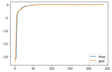
And now I can try implementing different ways to compute similarity. This is the log probability of the point being within the article space. That means that a larger value is better (larger meaning value closer to zero). All outputs are expected to be negative as the probability should never exceed 1.

Code

import numpy as np
from scipy.special import softmax
from scipy.stats import norm

def log_p(article: ArticleDescription, point: np.array, permutation: float = 0.01) -> float:
    """ Calculates the log probability of
    this feature describing the provided point.
    The point values are assumed to come straight
    from the model without softmax being applied. """

    point = softmax(point)
    point = point[article.indices]

    left_cdf = norm.cdf(
        point - permutation,
        loc=article.mean,
        scale=article.std,
    )
    right_cdf = norm.cdf(
        point + permutation,
        loc=article.mean,
        scale=article.std,
    )
    local_probability = right_cdf - left_cdf

    # there can be points where the probability is zero
    # because they are that far out of the distribution
    local_probability[local_probability <= 0] = 1e-9

    return np.log(local_probability)

I’ve worked over this a few times and I’ve finally got something I’m reasonably happy with. The code seems clean and I can justify each step of it.

Code

target_description = ArticleDescription.make(label="target corporation", df=target_corporation_df)

Code

print(f"target (shop) mean: {log_p(target_description, target_shop_output).sum()}")
print(f"target (goal) mean: {log_p(target_description, target_goal_output).sum()}")

target (shop) mean: -165.81268293270875
target (goal) mean: -61.83970056510085

Code

print(f"target (shop) minimum: {log_p(target_description, target_shop_output).min()}")
print(f"target (goal) minimum: {log_p(target_description, target_goal_output).min()}")

target (shop) minimum: -33.64575811631879
target (goal) minimum: -12.242802054947655

Code

import pandas as pd

pd.DataFrame({
    "shop": pd.Series(log_p(target_description, target_shop_output))
        .sort_values()
        .reset_index(drop=True),
    "goal": pd.Series(log_p(target_description, target_goal_output))
        .sort_values()
        .reset_index(drop=True),
}).plot() ; None

Well this has immediately failed. The shop output is considered dramatically less likely to be within the space than the goal meaning. It seems that the shop suffers from some very low probability tokens which skew the entire output.

Is my core assumption here correct? Is this approach to measuring containment within a cluster effective?

I could measure similarity to the cluster by taking the dot product or cosine similarity. A boundary could be established by working out the variance across the different tokens and then scaling them to unit length. Then (scaled) euclidean distance could be used as a measure.

Distance Measurement

For distance a lower score is better as we are measuring how close the point is to the center of the cluster.

Code

from scipy.special import softmax
from scipy.spatial.distance import euclidean
import numpy as np

def distance(article: ArticleDescription, point: np.array) -> float:
    """ Calculates the euclidean distance between
    the point and the cluster centroid. """

    point = softmax(point)
    point = point[article.indices]

    return euclidean(point, article.mean)

def distance_weighted(article: ArticleDescription, point: np.array) -> float:
    """ Calculates the euclidean distance between
    the point and the cluster centroid. """

    point = softmax(point)
    point = point[article.indices]

    return euclidean(point, article.mean, w=1/article.std)

Code

print(f"target (shop) distance: {distance(target_description, target_shop_output)}")
print(f"target (goal) distance: {distance(target_description, target_goal_output)}")

target (shop) distance: 0.25349703285833175
target (goal) distance: 0.24292873170701107

This is still failing. I wonder if scaling the distances by the std would help?

Code

print(f"target (shop) weighted distance: {distance_weighted(target_description, target_shop_output)}")
print(f"target (goal) weighted distance: {distance_weighted(target_description, target_goal_output)}")

target (shop) weighted distance: 2.457814269669948
target (goal) weighted distance: 1.4695577745700033

Nope. Fundamentally is this shop point even within the cluster?

Cosine Similarity

This is a measure of the similarity between the two vector angles. It is traditionally scaled between 1 (exactly identical angle) and -1 (exactly opposite angle). A value of 0 means the two vectors are orthogonal.

It turns out that scipy has implemented it such that two identical vector directions produce a result of 0, orthogonal is now 1 and opposite is 2.

Code

from scipy.spatial.distance import cosine

print(f"cosine similarity for same direction:       {cosine([0, 1], [0, 100])}")
print(f"cosine similarity for orthogonal direction: {cosine([0, 1], [1, 0])}")
print(f"cosine similarity for opposite direction:   {cosine([0, 1], [0, -1])}")

cosine similarity for same direction:       0
cosine similarity for orthogonal direction: 1.0
cosine similarity for opposite direction:   2.0

If this works then the shop value should be closer to zero than the goal value.

Code

from scipy.special import softmax
from scipy.spatial.distance import cosine
import numpy as np

def cosine_similarity(article: ArticleDescription, point: np.array) -> float:
    """ Calculates the dot product between the point and the mean. """

    point = softmax(point)
    point = point[article.indices]

    return cosine(point, article.mean)

def cosine_similarity_weighted(article: ArticleDescription, point: np.array) -> float:
    """ Calculates the dot product between the point and the mean. """

    point = softmax(point)
    point = point[article.indices]

    return cosine(point, article.mean, w=1/article.std)

Code

print(f"target (shop) cosine similarity: {cosine_similarity(target_description, target_shop_output)}")
print(f"target (goal) cosine similarity: {cosine_similarity(target_description, target_goal_output)}")

target (shop) cosine similarity: 0.7037042245833542
target (goal) cosine similarity: 0.8114881296160947

Code

print(f"target (shop) weighted cosine similarity: {cosine_similarity_weighted(target_description, target_shop_output)}")
print(f"target (goal) weighted cosine similarity: {cosine_similarity_weighted(target_description, target_goal_output)}")

target (shop) weighted cosine similarity: 0.6752133441786808
target (goal) weighted cosine similarity: 0.6246430215541248

Yeah that’s a no. The weighted one is incorrect and the unweighted version are very close to each other. Shop is closer to being orthogonal than identical.

Dot Product

This is the sum of the indexwise products, so a larger score is better. It’s another distance measurement and someone suggested it was equivalent to cosine similarity.

Code

from scipy.special import softmax
import numpy as np

def dot(article: ArticleDescription, point: np.array) -> float:
    """ Calculates the dot product between the point and the mean. """

    point = softmax(point)
    point = point[article.indices]

    return np.dot(point, article.mean)

def dot_weighted(article: ArticleDescription, point: np.array) -> float:
    """ Calculates the dot product between the point and the mean. """

    point = softmax(point)
    point = point[article.indices]

    return np.sum(np.multiply(point, article.mean) / article.std)

Code

print(f"target (shop) dot product: {dot(target_description, target_shop_output)}")
print(f"target (goal) dot product: {dot(target_description, target_goal_output)}")

target (shop) dot product: 0.012649087921898306
target (goal) dot product: 0.004475755772202107

Code

print(f"target (shop) weighted dot product: {dot_weighted(target_description, target_shop_output)}")
print(f"target (goal) weighted dot product: {dot_weighted(target_description, target_goal_output)}")

target (shop) weighted dot product: 1.1805841145809688
target (goal) weighted dot product: 0.621057388615067

FINALLY.

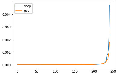
I would need a way to threshold this to determine containment, but at least there is a significant difference between these two scores. It’s interesting that weighting the products actually brings the two scores closer together (moves towards a 2x difference instead of a 3x difference).

Code

import pandas as pd

pd.DataFrame({
    "shop": pd.Series(
            np.multiply(
                softmax(target_shop_output[target_description.indices]),
                target_description.mean
            )
        )
        .sort_values()
        .reset_index(drop=True),
    "goal": pd.Series(
            np.multiply(
                softmax(target_goal_output[target_description.indices]),
                target_description.mean
            )
        )
        .sort_values()
        .reset_index(drop=True),
}).plot() ; None

It seems that the sum over the product has the same shape as the log probability, except in this case it works in favour of the shop classification.

I’m mindful that this is testing a single article description against a pair of outputs. To properly evaluate this I need a far broader dataset. More immediately I need the scores to be comparable at all.

The dot product between 200 tokens will likely be larger than one between 100 tokens. This is because every elementwise product will be positive and so it will roughly scale with the number of tokens. If I take the mean of the products then a description with more tokens is likely to have a lower score than one with less. This is due to the shape of the token scores - they go through softmax so there will be power law shape over the token scores. As more tokens are included the token scores will drop and so the additional products will be much lower.

What I could do is take the top N scores after the product and sum them. That would at least be consistent as I could ensure that every article has at least that many scores.

Code

def dot_filtered(article: ArticleDescription, point: np.array, n: int = 10) -> float:
    """ Calculates the dot product between the point and the mean. """

    point = softmax(point)
    point = point[article.indices]
    product = np.multiply(point, article.mean)

    # np.sort is ascending
    return np.sum(np.sort(product)[-n:])

def dot_weighted_filtered(article: ArticleDescription, point: np.array, n: int = 10) -> float:
    """ Calculates the dot product between the point and the mean. """

    point = softmax(point)
    point = point[article.indices]
    product = np.multiply(point, article.mean) / article.std

    # np.sort is ascending
    return np.sum(np.sort(product)[-n:])

Code

print(f"target (shop) filtered dot product: {dot_filtered(target_description, target_shop_output)}")
print(f"target (goal) filtered dot product: {dot_filtered(target_description, target_goal_output)}")

target (shop) filtered dot product: 0.010653895085615227
target (goal) filtered dot product: 0.003070220959723772

Code

print(f"target (shop) weighted filtered dot product: {dot_weighted_filtered(target_description, target_shop_output)}")
print(f"target (goal) weighted filtered dot product: {dot_weighted_filtered(target_description, target_goal_output)}")

target (shop) weighted filtered dot product: 0.6238547218338613
target (goal) weighted filtered dot product: 0.2011766823443498

This works out well as it preserves the relative ratio between the scores of around 3x and it should be more comparable between different articles. I am not sure about the approach of weighting the dot product as we are not measuring the similarity to the target point anymore. The weighting approach boosts those tokens that have a very restricted range in the article even if the value from the point is wildly outside that range.

As such I think the base dot product is more justifiable.

Eigenvalue

A co-worker pointed out that PCA generates the eigenvectors that can be used to remap the values. If I run PCA over the feature points then I could come up with maybe 10 eigenvectors. The mean and std of those would then make for a better description of the cluster as they would be aligned with the major dimensions.

Code

from __future__ import annotations
from dataclasses import dataclass

from scipy.special import softmax
from scipy.spatial.distance import cosine, euclidean
from scipy.stats import norm
from sklearn.decomposition import PCA
import numpy as np

@dataclass
class ArticleEigenDescription:
    label: str
    indices: np.array
    covariance: np.array
    mean: np.array
    std: np.array

    def make(label: str, df: pd.DataFrame, minimum_count: int = 5, dimensions: int = 10) -> ArticleDescription:
        token_probability_df = pd.DataFrame(
            df.apply(
                lambda row: dict(zip(row["index"], row["probability"])),
                axis="columns"
            ).tolist()
        )
        # sort token columns, which leads to sorted indices/mean/std values
        token_probability_df = token_probability_df[np.sort(token_probability_df.columns)]

        # drop any columns which do not have at least minimum_count values
        column_mask = (~token_probability_df.isna()).sum(axis="rows") >= minimum_count
        column_names = column_mask[column_mask].index # the column names where the mask is true
        token_probability_df = token_probability_df[column_names]
        token_probability_df = token_probability_df.fillna(0)

        indices = token_probability_df.columns.to_numpy()
        token_probability_np = token_probability_df.to_numpy()

        # remap everything through PCA
        pca = PCA(
            n_components=dimensions,
            random_state=0,
        )
        transformed_probability = pca.fit_transform(token_probability_np)
        covariance = pca.components_

        mean = np.mean(transformed_probability, axis=0)
        std = np.std(transformed_probability, axis=0)

        return ArticleEigenDescription(
            label=label,
            indices=indices,
            covariance=covariance,
            mean=mean,
            std=std,
        )

    def describe(self, point: np.array) -> dict[str, float]:
        return {
            "cosine_unweighted": self.cosine_similarity(point),
            "cosine_weighted": self.cosine_similarity(point, weight=True),
            "distance_unweighted": self.distance(point),
            "distance_weighted": self.distance(point, weight=True),
            "dot_unweighted": self.dot(point),
            "dot_weighted": self.dot(point, weight=True),
            "log_p_mean": self.log_p(point).mean(),
            "log_p_min": self.log_p(point).min(),
        }

    def transform(self, point: np.array) -> np.array:
        point = softmax(point)
        point = point[self.indices]
        point = self.covariance @ point
        return point

    def cosine_similarity(self, point: np.array, weight: bool = False) -> float:
        """ Calculates the dot product between the point and the mean.
        This returns 0. for identical direction, 1 for orthogonal and 2 for opposite. """
        point = self.transform(point)
        return cosine(point, self.mean, w=1/self.std if weight else None)

    def distance(self, point: np.array, weight: bool = False) -> float:
        """ Calculates the euclidean distance between
        the point and the cluster centroid. """
        point = self.transform(point)
        return euclidean(point, self.mean, w=1/self.std if weight else None)

    def dot(self, point: np.array, weight: bool = False) -> float:
        """ Calculates the dot product between the point and the mean. """
        point = self.transform(point)
        if not weight:
            return np.dot(point, self.mean)
        return np.sum(np.multiply(point, self.mean) / self.std)

    def log_p(self, point: np.array, permutation: float = 0.01) -> float:
        """ Calculates the log probability of
        this feature describing the provided point.
        The point values are assumed to come straight
        from the model without softmax being applied. """
        point = self.transform(point)

        left_cdf = norm.cdf(
            point - permutation,
            loc=self.mean,
            scale=self.std,
        )
        right_cdf = norm.cdf(
            point + permutation,
            loc=self.mean,
            scale=self.std,
        )
        local_probability = right_cdf - left_cdf

        # there can be points where the probability is zero
        # because they are that far out of the distribution
        local_probability[local_probability <= 0] = 1e-9

        return np.log(local_probability)

Code

target_eigen_description = ArticleEigenDescription.make(label="target corporation", df=target_corporation_df, minimum_count=20)

Code

pd.DataFrame(
    [
        target_eigen_description.describe(target_shop_output),
        target_eigen_description.describe(target_goal_output),
    ],
    index=["shop", "goal"]
)

	cosine_unweighted	cosine_weighted	distance_unweighted	distance_weighted	dot_unweighted	dot_weighted	log_p_mean	log_p_min
shop	0.477628	0.610804	0.067580	0.365985	5.467629e-19	8.898288e-18	-1.905805	-2.915850
goal	1.151482	1.437208	0.027011	0.159297	-6.337334e-20	-4.350816e-18	-1.676546	-2.639569

I’m very surprised by the dot product values. The cosine similarity scores are way way better now.

Code

np.abs(target_eigen_description.covariance).mean(axis=1)

array([0.02297287, 0.02401784, 0.02242427, 0.02007332, 0.03257951,
       0.02410345, 0.02789364, 0.02818695, 0.03248836, 0.04065791])

Code

target_eigen_description.transform(target_shop_output)

array([ 0.00644708,  0.04052714,  0.01465268, -0.02805793,  0.00028818,
        0.02423663, -0.005811  , -0.00765501,  0.00674133, -0.03399733])

Code

target_eigen_description.transform(target_goal_output)

array([ 0.0039489 ,  0.00900655, -0.00506472,  0.00187765, -0.01479912,
        0.00418708,  0.01231673, -0.00587802, -0.00873955,  0.01022457])

Code

np.abs(target_eigen_description.mean).mean()

3.731339670899627e-18

The problem seems to be that the mean of the point values is low and the mean itself is low. If the average feature value becomes ~1e-2 after being mapped to 10 features, and the mean of the article values is ~1e-18 then the resulting product will be ~1e-20.

Fixing this would just require scaling the values appropriately. That would alter some of the other metrics like log_p and distance so I’m only going to do it if it is worthwhile.

As it is this looks far more promising. The probability approach is still broken but the others all now distinguish between the two sentences correctly. I’m quite interested in cosine and dot product as they both have quite nice properties - the cosine value has a possible cut off point somewhere before 1 and the dot product now seems to produce positive and negative values.

This is certainly an improvement. Let’s see how it does against a larger set of sentences.