Perceptual Advert Blocking

I recently read a paper about using deep learning to block images containing adverts (Din et al. 2019). The novelty of the paper appears to be the specific classification domain, the size of the model (very small at 1.76MB), and the integration of the blocker directly into the browser. Given that the image classifier seems quite simple (a variant of SqueezeNet (Iandola et al. 2016)) which is quite old now, I wonder if I can reproduce this using CLIP.

Din, Zain ul abi, Panagiotis Tigas, Samuel T. King, and Benjamin Livshits. 2019. “Percival: Making in-Browser Perceptual Ad Blocking Practical with Deep Learning.” arXiv. https://doi.org/10.48550/ARXIV.1905.07444.

Iandola, Forrest N., Song Han, Matthew W. Moskewicz, Khalid Ashraf, William J. Dally, and Kurt Keutzer. 2016. “SqueezeNet: AlexNet-Level Accuracy with 50x Fewer Parameters and ≪0.5MB Model Size.” arXiv. https://doi.org/10.48550/ARXIV.1602.07360.

The first thing to do will be to collect the dataset. Then I can try clustering it using the CLIP embeddings to find out how many separate classifiers I should use. Finally I can evaluate the classifier embeddings against a separate dataset.

Dataset

One problem is that the dataset does not seem to be available. I’ve found a dataset of 64,832 adverts in the Pitt Image Ads Dataset (can’t seem to find citation, it’s by Adriana Kovashka and is available here). I can use this with the open images dataset that I already have.

Let’s have a look at one of the images first:

Code

from pathlib import Path

ADVERT_FOLDER = Path("/data/image/pitt_adverts/image/")
ADVERT_IMAGES = sorted(ADVERT_FOLDER.glob("*/*"))

DATA_FOLDER = Path("/data/blog/2022/11/29/perceptual-adblocking")
DATA_FOLDER.mkdir(exist_ok=True, parents=True)

Code

from pathlib import Path
from PIL import Image

Image.open(ADVERT_IMAGES[0])

My real dataset is the embeddings for all of these images. Let’s create them.

Code

from pathlib import Path
from PIL import Image
import numpy as np
import torch
from transformers import CLIPProcessor, CLIPModel

model = CLIPModel.from_pretrained("openai/clip-vit-base-patch32")
processor = CLIPProcessor.from_pretrained("openai/clip-vit-base-patch32")

@torch.inference_mode()
def calculate_embedding(file: Path) -> np.array:
    image = Image.open(file)
    image_features = processor.feature_extractor(image, return_tensors="pt")
    vision_outputs = model.vision_model(**image_features)
    image_embeds = model.visual_projection(vision_outputs.pooler_output)
    return image_embeds.numpy()[0]

Code

from tqdm.auto import tqdm
import pandas as pd

advert_embedding_df = pd.DataFrame([
    {
        "file": str(file.relative_to(ADVERT_FOLDER)),
        "embedding": calculate_embedding(file),
    }
    for file in tqdm(ADVERT_IMAGES)
])
advert_embedding_df.to_parquet(DATA_FOLDER / "advert-embeddings.gz.parquet", compression="gzip")

advert_embedding_df

	file	embedding	label
0	0/10000.jpg	[0.15955794, 0.12757635, -0.1171277, -0.125003...	0
1	0/100000.jpg	[-0.26774788, -0.18349923, 0.03581748, 0.01433...	0
2	0/100010.jpg	[-0.54049927, -0.0582103, -0.32849184, -0.2700...	1
3	0/100040.jpg	[-0.63116956, -0.1476591, -0.035523407, -0.383...	0
4	0/100060.jpg	[-0.18007469, 0.18109158, 0.054699436, 0.22198...	1
...	...	...	...
64827	9/99899.jpg	[-0.17220578, 0.056135595, -0.054074608, -0.41...	0
64828	9/99959.jpg	[0.15200219, -0.09595037, -0.08600271, 0.65402...	2
64829	9/99969.jpg	[-0.20257103, -0.38640052, 0.14894253, -0.1454...	1
64830	9/99979.jpg	[0.022974648, -0.5470357, -0.22149833, -0.1679...	2
64831	9/99989.jpg	[0.1348732, -0.54329157, 0.16097397, 0.3252397...	1

64832 rows × 3 columns

Clustering

The next thing is to try to define embeddings that can be used to identify the adverts. A nice way to do this is to cluster the embeddings and use the cluster centroids as classifiers - if a new embedding is near to a cluster centroid then we can label the image as an advert.

With CLIP the normal way to measure label / image similarity is to use cosine similarity. SKLearn can be used to create KMeans clusters. If the embeddings are normalized then the KMeans clusters will be defined over the cosine similarity of the embeddings.

To work with this we must ensure that the embeddings are normalized, as that will make the mean square metric into the cosine similarity metric for KMeans.

from sklearn import preprocessing
import numpy as np

X = np.array(advert_embedding_df.embedding.tolist())
X = preprocessing.normalize(X)
(X*X).sum(axis=1).mean()

1.0

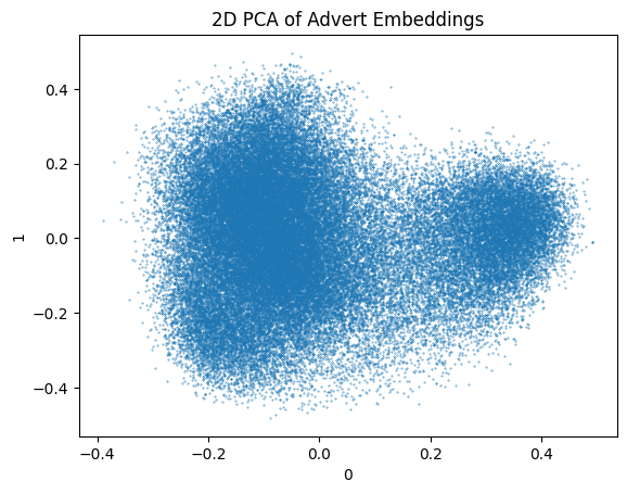
KMeans is nice however to use it we have to know how many clusters are present in the data. If we visualize it we might have an idea. I’ve used PCA and T-SNE before to do this so let’s use them again.

Code

from sklearn.decomposition import PCA

pca_output = PCA(
    n_components=2,
    random_state=0,
).fit_transform(X)
pca_df = pd.DataFrame(pca_output)

pca_df.plot.scatter(
    title="2D PCA of Advert Embeddings",
    x=0,
    y=1,
    s=0.1,
) ; None

Code

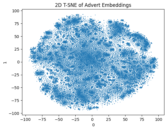
from sklearn.decomposition import PCA
from sklearn.manifold import TSNE
import numpy as np

n_components = 2

# doing this to avoid the warning about future T-SNE
tsne_init = (
    PCA(
        n_components=n_components,
        svd_solver="randomized",
        random_state=0,
    )
        .fit_transform(X)
        .astype(np.float32, copy=False)
)

tsne_output = TSNE(
    n_components=n_components,
    learning_rate="auto",
    init=tsne_init,
).fit_transform(X)

tsne_df = pd.DataFrame(tsne_output)
tsne_df.plot.scatter(
    title="2D T-SNE of Advert Embeddings",
    x=0,
    y=1,
    s=0.1,
) ; None

Here we can see that the PCA visualization has not clearly separated the points. There is perhaps two clusters in that. T-SNE is significantly slower and shows far more variation in the data. There could be hundreds of distinct clusters in that.

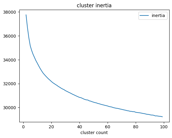
Another way to determine the cluster count is to use the elbow method, where you plot the distortion and inertia. Distortion is the mean of the squared distance for each point to the center of the cluster. Inertia is the sum of the squared distance for each point to the center of the nearest other cluster. The “elbow” comes from the point in the graph where the rate of change of these values suddenly changes.

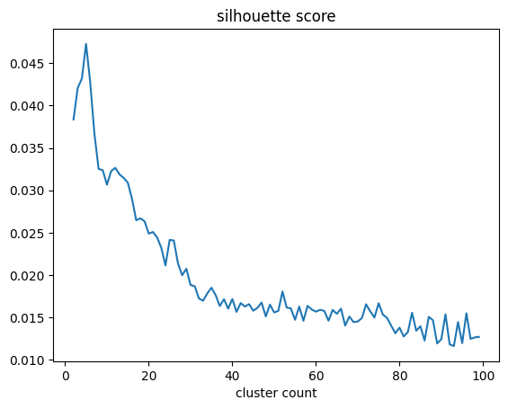
I’ve recently heard of the silhouette score which is a metric based on the distortion and inertia. You can calculate it for each cluster count and then take the count with the highest number. I like this as it automates the elbow.

Code

from tqdm.auto import tqdm
import pandas as pd
from sklearn.cluster import KMeans
from sklearn.metrics import silhouette_score

def cluster_score(X: np.array, n_clusters: int) -> float:
    kmeans = KMeans(
        n_clusters=n_clusters,
        random_state=42,
    )
    labels = kmeans.fit_predict(X)
    score = silhouette_score(X, labels)
    return score

cluster_df = pd.DataFrame([
    {
        "clusters": n_clusters,
        "score": cluster_score(X, n_clusters=n_clusters),
    }
    for n_clusters in tqdm(range(2, 100))
])
(
    cluster_df
        .set_index("clusters")
        .score
        .plot(title="silhouette score", xlabel="cluster count")
) ; None

Code

from tqdm.auto import tqdm
import pandas as pd
from sklearn.cluster import KMeans
from sklearn.metrics import silhouette_score

def cluster_score(X: np.array, n_clusters: int) -> dict[str, float]:
    kmeans = KMeans(
        n_clusters=n_clusters,
        random_state=42,
    )
    labels = kmeans.fit_predict(X)
    return {
        "cluster_count": n_clusters,
        "inertia": kmeans.inertia_,
    }

cluster_df = pd.DataFrame([
    cluster_score(X, n_clusters=n_clusters)
    for n_clusters in tqdm(range(2, 100))
])
(
    cluster_df
        .set_index("cluster_count")
        .plot(title="cluster inertia", xlabel="cluster count")
) ; None

The silhouette method suggests that there are 5 clusters, while the elbow method is less conclusive. I was expecting more as the original CLIP paper used 80 templates per class.

The next thing to do is to make a classifier out of this and see how many of the open images get classified as adverts.

Code

from tqdm.auto import tqdm
import pandas as pd
from sklearn.cluster import KMeans

CLUSTER_COUNT = 5

def cluster_centroids(X: np.array, n_clusters: int) -> np.array:
    kmeans = KMeans(
        n_clusters=n_clusters,
        random_state=42,
    )
    kmeans.fit(X)
    return kmeans.cluster_centers_, kmeans.labels_

centroids, labels = cluster_centroids(X, n_clusters=CLUSTER_COUNT)
advert_embedding_df["label"] = labels

advert_embedding_df.to_parquet(
    DATA_FOLDER / "labelled-advert-embeddings.gz.parquet",
    compression="gzip",
)

One problem with this is that the different clusters may have different variance. I want to be able to train a classification head using these centroids as a starting point. Then the bias over that linear layer can be used to set the size of the cluster.

Classifying

With a classification layer that uses the centroids as the starting weights how well can I classify this existing dataset? I can create a model which uses the CLIP stages first to produce the embedding, then uses a linear layer to classify the image into one of the 5 clusters. This linear layer can be initialized with the cluster centroids that we have just calculated.

A model structured in this way should work as the linear layer is reproducing the dot product. If we want to recreate cosine similarity exactly then normalizing the model output prior to the linear layer will do this. Otherwise we can use an adjusted sigmoid following the classification, and in this way the range of output remains -1 to 1 in both cases.

Code

from typing import Union
from pathlib import Path

from PIL import Image
import numpy as np
from torch import nn
import torch
import torch.nn.functional as F
from transformers import CLIPProcessor, CLIPModel

class CLIPClassifier(nn.Module):
    def __init__(
        self,
        processor: CLIPProcessor,
        model: CLIPModel,
        centroids: np.array,
        normalize: bool = True,
    ) -> None:
        super().__init__()
        self.feature_extractor = processor.feature_extractor
        self.vision_model = model.vision_model
        self.visual_projection = model.visual_projection
        out_features, in_features = centroids.shape
        classifier = nn.Linear(
            in_features=in_features,
            out_features=out_features,
            bias=True,
        )
        classifier.weight.data = torch.from_numpy(centroids).clone()
        self.bias = classifier.bias
        if normalize:
            self.classifier = nn.Sequential(
                NormalizeLayer(),
                classifier
            )
        else:
            self.classifier = nn.Sequential(
                classifier,
                AdjustedSigmoid(),
            )

    def infer(self, image: Union[Path, str, Image.Image]) -> float:
        if not isinstance(image, Image.Image):
            image = Image.open(image)
        image_features = self.feature_extractor(
            image, return_tensors="pt",
        )
        return self(**image_features)

    def forward(self, pixel_values: torch.Tensor) -> torch.Tensor:
        vision_outputs = self.vision_model(pixel_values=pixel_values)
        image_embeds = self.visual_projection(vision_outputs.pooler_output)
        return self.classifier(image_embeds)

class NormalizeLayer(nn.Module):
    def forward(self, inputs: torch.Tensor) -> torch.Tensor:
        return F.normalize(inputs, dim=-1)

class AdjustedSigmoid(nn.Module):
    def forward(self, inputs: torch.Tensor) -> torch.Tensor:
        return torch.sigmoid(inputs) * 2 - 1

We can now see what this classifier would produce without any training. The only thing that is untrained is the bias, which tends to be low to start with.

classifier = CLIPClassifier(
    processor=CLIPProcessor.from_pretrained("openai/clip-vit-base-patch32"),
    model=CLIPModel.from_pretrained("openai/clip-vit-base-patch32"),
    centroids=centroids,
    normalize=True,
)

with torch.inference_mode():
    output = classifier.infer(
        ADVERT_FOLDER / advert_embedding_df.iloc[0].file
    )

print(f"predictions: {output[0]}")
print(f"image cluster: {advert_embedding_df.iloc[0].label}")

predictions: tensor([0.5483, 0.4682, 0.3830, 0.4260, 0.4176])
image cluster: 0

The output is strongly positive for all of the classes. What I want to do now is to train only the bias to calibrate it.

Training

My training approach will be as follows:

• Embed an equal number of “non” advert images from my openimages dataset
• For a non advert image I want every class output to be zero or below
• For every advert image I want the associated output to be above zero
• Advert images do not train the other classifier biases, they can be above or below zero

I should get cracking with this as it should be quite a quick train. It’s going to take longer to generate the embeddings for the open images dataset.

Code

from pathlib import Path

OPENIMAGES_FOLDER = Path("/data/image/open-images/images/train_0/")
OPENIMAGES_IMAGES = sorted(OPENIMAGES_FOLDER.glob("*.jpg"))

LEARNING_RATE = 1.5e-3
EPOCHS = 10
BATCH_SIZE = 256

MODEL_RUN_FOLDER = Path("/data/blog/2022/11/29/perceptual-adblocking/runs")
MODEL_RUN_FOLDER.mkdir(parents=True, exist_ok=True)

from tqdm.auto import tqdm
import pandas as pd

openimages_embedding_df = pd.DataFrame([
    {
        "file": str(file.relative_to(OPENIMAGES_FOLDER)),
        "embedding": calculate_embedding(file),
    }
    for file in tqdm(OPENIMAGES_IMAGES[:len(ADVERT_IMAGES)])
])
openimages_embedding_df.to_parquet(
    DATA_FOLDER / "non-advert-embeddings.gz.parquet",
    compression="gzip",
)

openimages_embedding_df

	file	embedding
0	000002b66c9c498e.jpg	[-0.06684355, 0.109889895, -0.07951541, 0.3099...
1	000002b97e5471a0.jpg	[-0.009899404, -0.2985628, -0.026171125, 0.104...
2	000002c707c9895e.jpg	[0.49510366, 0.280301, 0.13652878, 0.12522303,...
3	0000048549557964.jpg	[-0.4103726, 0.044636518, -0.32004184, 0.32154...
4	000004f4400f6ec5.jpg	[0.23297504, 0.12402086, -0.20056993, 0.102245...
...	...	...
64827	04f3060b8c58a5a3.jpg	[-0.17162555, -0.09748538, -0.07931266, 0.4867...
64828	04f31161fdd55209.jpg	[-0.14677836, 0.05942069, -0.04285209, 0.54772...
64829	04f3167d8bf1b627.jpg	[-0.3469041, -0.108701, -0.26653805, 0.3233778...
64830	04f3210f9764509c.jpg	[-0.25462195, 0.4342759, -0.09380726, -0.04035...
64831	04f32a3ca353ae53.jpg	[-0.4824751, 0.19964725, -0.12897669, 0.249913...

64832 rows × 2 columns

Code

from typing import Tuple
from sklearn.model_selection import train_test_split
import pandas as pd

def split_df(
    advert_df: pd.DataFrame,
    non_advert_df: pd.DataFrame,
    test_size: int = 100,
) -> Tuple[pd.DataFrame, pd.DataFrame]:
    advert_train, advert_test = train_test_split(
        advert_df,
        test_size=test_size // 2,
        random_state=42,
    )
    non_advert_df = non_advert_df.copy()
    non_advert_df["label"] = -1
    non_advert_train, non_advert_test = train_test_split(
        non_advert_df,
        test_size=test_size // 2,
        random_state=42,
    )
    train_df = pd.concat([
        advert_train,
        non_advert_train,
    ])
    test_df = pd.concat([
        advert_test,
        non_advert_test,
    ])
    return train_df, test_df

train_df, test_df = split_df(
    advert_df=advert_embedding_df,
    non_advert_df=openimages_embedding_df,
    test_size=1_000,
)
train_df.to_parquet(DATA_FOLDER / "train.gz.parquet", compression="gzip")
test_df.to_parquet(DATA_FOLDER / "test.gz.parquet", compression="gzip")

The dataset for these is then the desired output class and the embeddings. We know that the embeddings come directly from CLIP output, so running CLIP again doesn’t add much value.

The first thing to do is to define a loss function. This will control how the optimizer updates the bias of the classifier, so it is the most important thing to get right.

I have written this loss function to adhere to these principles:

• We can use sigmoid to map the outputs to a fixed range (will adjust it to be -1 to 1).
• For an advert we are only concerned with the output of the cluster index, that must be positive. Closer to 1 is better.
• For a non advert we want all outputs to be negative. Closer to -1 is better.
• We have an equal number of non adverts as adverts, so we don’t want a non advert to have more influence over the model than an advert.
• So the non advert will consider a random output instead of all of the outputs.

Code

from typing import Callable
import torch

LossFunction = Callable[[torch.Tensor, torch.Tensor], torch.Tensor]

def absolute_loss(outputs: torch.Tensor, labels: torch.Tensor) -> torch.Tensor:
    """
    This wants to move the outputs to +1 or -1.
    For a negative row one target is chosen at random to update.
    """
    labels = labels.clone()

    batch_size, label_count = outputs.shape
    indexes = labels
    index_mask = indexes == -1
    
    # target is the desired output value
    targets = torch.ones_like(indexes, device=outputs.device)
    targets[index_mask] *= -1
    
    # where the correct output is -1, we choose a random output index to test
    # this ensures that one negative example has the same influence as one positive example
    # and it provides a similar influence over the bias values
    indexes[index_mask] = torch.randint(
        low=0,
        high=label_count,
        size=(index_mask.sum(),),
        device=outputs.device,
    )
    outputs = outputs[range(batch_size), indexes]
    
    # the loss is based on the difference between the target and the output
    # this doesn't compare across all of the outputs at any point (which would allow cross entropy)
    # that is because if the image is an advert then it is fine for any output to be positive,
    # so other indices that are positive should not be punished
    loss = targets - outputs
    loss = loss**2
    loss = loss.sum()

    return loss

Next is to define a training loop and metric. This is quite verbose, normally we would be using the huggingface trainer however this is quite a specific task and doesn’t really fit into that.

Code

from typing import Tuple
import pandas as pd
import numpy as np
import torch
from torch.optim import Adam, Optimizer
from torch.optim.lr_scheduler import LinearLR, SequentialLR
from tqdm.auto import tqdm
from sklearn.model_selection import train_test_split
from IPython.display import update_display, display
import time
import math

def train(
    model: CLIPClassifier,
    train_df: pd.DataFrame,
    test_df: pd.DataFrame,
    lr: float,
    epochs: int,
    loss_fn: LossFunction,
    batch_size: int = 64,
    device: str = "cuda",
) -> pd.DataFrame:
    model.to(device)
    results_df = None
    df_display_id = f"train-results-{time.time()}"

    steps = int(math.ceil(len(train_df) / batch_size) * epochs)
    transition_step = int(steps * 0.06) + 1

    optimizer = Adam(params=[model.bias], lr=lr)
    scheduler = SequentialLR(
        optimizer,
        schedulers=[
            LinearLR(optimizer, start_factor=1/3, end_factor=1, total_iters=transition_step),
            LinearLR(optimizer, start_factor=1, end_factor=0, total_iters=steps-transition_step),
        ],
        milestones=[transition_step]
    )
    
    for epoch in tqdm(range(epochs)):
        train_loss = train_model(
            model=model,
            optimizer=optimizer,
            scheduler=scheduler,
            df=train_df,
            batch_size=batch_size,
            device=device,
            loss_fn=loss_fn,
        )
        test_loss, test_accuracy = test_model(
            model=model,
            df=test_df,
            batch_size=batch_size,
            device=device,
            loss_fn=loss_fn,
        )
        if results_df is None:
            results_df = pd.DataFrame([
                {
                    "epoch": epoch,
                    "train loss": train_loss,
                    "test loss": test_loss,
                    "accuracy": test_accuracy,
                }
            ])
            results_df = results_df.set_index("epoch")
            display(results_df, display_id=df_display_id)
        else:
            results_df.loc[epoch] = {
                "train loss": train_loss,
                "test loss": test_loss,
                "accuracy": test_accuracy,
            }
            update_display(results_df, display_id=df_display_id)

    return results_df

def train_model(
    model: CLIPClassifier,
    optimizer: Optimizer,
    scheduler,
    df: pd.DataFrame,
    batch_size: int,
    device: str,
    loss_fn: LossFunction,
) -> float:
    train_loss = 0
    model.train()
    shuffled = df.sample(frac=1)
    for index in tqdm(range(0, len(shuffled), batch_size), leave=False):
        embeddings, labels = to_batch(df, index=index, batch_size=batch_size, device=device)
        optimizer.zero_grad()
        outputs = model.classifier(embeddings)
        loss = loss_fn(outputs, labels)
        loss.backward()
        optimizer.step()
        scheduler.step()
        train_loss += loss.item()
    return train_loss / len(shuffled)

@torch.no_grad()
def test_model(
    model: CLIPClassifier,
    df: pd.DataFrame,
    batch_size: int,
    device: str,
    loss_fn: LossFunction,
) -> Tuple[float, float]:
    test_loss = 0
    test_accuracy = 0
    model.eval()
    for index in tqdm(range(0, len(df), batch_size), leave=False):
        embeddings, labels = to_batch(df, index=index, batch_size=batch_size, device=device)
        outputs = model.classifier(embeddings)
        loss = loss_fn(outputs, labels)
        accuracy = accuracy_fn(outputs, labels)
        test_loss += loss.item()
        test_accuracy += accuracy.item()
    return test_loss / len(df), test_accuracy / len(df)

def to_batch(
    df: pd.DataFrame,
    index: int,
    batch_size: int,
    device: str,
) -> Tuple[torch.Tensor, torch.Tensor]:
    rows = df.iloc[index:index+batch_size]
    embeddings = torch.from_numpy(
        np.array(rows.embedding.tolist())
    ).to(device)
    labels = torch.tensor(
        rows.label.tolist()
    ).to(device)
    return embeddings, labels

def accuracy_fn(outputs: torch.Tensor, labels: torch.Tensor) -> torch.Tensor:
    batch_size, label_count = outputs.shape
    max_values, _ = outputs.max(dim=1)
    index_mask = max_values >= 0
    label_mask = labels >= 0
    return (index_mask == label_mask).sum()

Train with Normalization

This adds the normalization to the model before the linear layer. Doing this makes the output of the linear layer the cosine similarity of the cluster centroids and the current embedding.

classifier = CLIPClassifier(
    processor=CLIPProcessor.from_pretrained("openai/clip-vit-base-patch32"),
    model=CLIPModel.from_pretrained("openai/clip-vit-base-patch32"),
    centroids=centroids,
    normalize=True,
)

train(
    model=classifier,
    train_df=train_df,
    test_df=test_df,
    lr=1.5e-3,
    epochs=20,
    batch_size=256,
    loss_fn=absolute_loss,
) ; None

	train loss	test loss	accuracy
epoch
0	1.001089	0.944663	0.496
1	0.893075	0.906864	0.501
2	0.891319	0.914037	0.517
3	0.901312	0.928193	0.546
4	0.907296	0.917159	0.542
5	0.911599	0.924555	0.541
6	0.914176	0.917649	0.540
7	0.913495	0.922158	0.521
8	0.914344	0.915177	0.507
9	0.914007	0.918570	0.502
10	0.913057	0.915863	0.499
11	0.912555	0.912235	0.505
12	0.911870	0.906080	0.507
13	0.910994	0.909880	0.503
14	0.910171	0.908032	0.499
15	0.909059	0.898542	0.490
16	0.908103	0.906639	0.488
17	0.907192	0.913889	0.490
18	0.905588	0.912610	0.491
19	0.904710	0.905274	0.493

/home/matthew/.local/share/virtualenvs/blog-1tuLwbZm/lib/python3.10/site-packages/torch/optim/lr_scheduler.py:156: UserWarning: The epoch parameter in `scheduler.step()` was not necessary and is being deprecated where possible. Please use `scheduler.step()` to step the scheduler. During the deprecation, if epoch is different from None, the closed form is used instead of the new chainable form, where available. Please open an issue if you are unable to replicate your use case: https://github.com/pytorch/pytorch/issues/new/choose.
  warnings.warn(EPOCH_DEPRECATION_WARNING, UserWarning)

classifier.to("cpu")

with torch.inference_mode():
    output = classifier.infer(ADVERT_FOLDER / advert_embedding_df.iloc[0].file)

print(f"predictions: {output[0]}")
print(f"image cluster: {advert_embedding_df.iloc[0].label}")

predictions: tensor([ 0.2086,  0.1007,  0.0850, -0.0677, -0.0987])
image cluster: 0

with torch.inference_mode():
    output = classifier.infer(OPENIMAGES_FOLDER / openimages_embedding_df.iloc[0].file)

print(f"predictions: {output[0]}")
print("no image cluster")

predictions: tensor([ 0.0059, -0.1296, -0.0508, -0.2039, -0.2314])
no image cluster

This is interesting. The training results in decreasing accuracy which I can’t seem to figure out. When running it over those two images the non advert image has been incorrectly classified.

Train without Normalization

This does not add the normalization to the model before the linear layer. When creating a model it can be good to avoid too much manipulation as that reduces the amount that the model can adjust itself. Let’s see if this works better.

classifier = CLIPClassifier(
    processor=CLIPProcessor.from_pretrained("openai/clip-vit-base-patch32"),
    model=CLIPModel.from_pretrained("openai/clip-vit-base-patch32"),
    centroids=centroids,
    normalize=False,
)

train(
    model=classifier,
    train_df=train_df,
    test_df=test_df,
    lr=1e-2,
    epochs=20,
    batch_size=256,
    loss_fn=absolute_loss,
) ; None

	train loss	test loss	accuracy
epoch
0	1.400746	0.819867	0.570
1	0.611357	1.032671	0.557
2	0.759185	1.016272	0.558
3	0.773477	0.986434	0.556
4	0.778775	0.969343	0.559
5	0.782921	0.946825	0.563
6	0.786529	0.930116	0.566
7	0.790562	0.914012	0.575
8	0.793381	0.895699	0.569
9	0.795106	0.881502	0.569
10	0.798442	0.866560	0.575
11	0.799043	0.850110	0.574
12	0.800381	0.840381	0.568
13	0.801248	0.831682	0.575
14	0.801238	0.818669	0.575
15	0.800040	0.809591	0.573
16	0.799471	0.811441	0.571
17	0.799041	0.815090	0.562
18	0.794730	0.795042	0.561
19	0.792499	0.804033	0.558

/home/matthew/.local/share/virtualenvs/blog-1tuLwbZm/lib/python3.10/site-packages/torch/optim/lr_scheduler.py:156: UserWarning: The epoch parameter in `scheduler.step()` was not necessary and is being deprecated where possible. Please use `scheduler.step()` to step the scheduler. During the deprecation, if epoch is different from None, the closed form is used instead of the new chainable form, where available. Please open an issue if you are unable to replicate your use case: https://github.com/pytorch/pytorch/issues/new/choose.
  warnings.warn(EPOCH_DEPRECATION_WARNING, UserWarning)

classifier.to("cpu")

with torch.inference_mode():
    output = classifier.infer(ADVERT_FOLDER / advert_embedding_df.iloc[0].file)

print(f"predictions: {output[0]}")
print(f"image cluster: {advert_embedding_df.iloc[0].label}")

predictions: tensor([0.6315, 0.4511, 0.4669, 0.2789, 0.1313])
image cluster: 0

with torch.inference_mode():
    output = classifier.infer(OPENIMAGES_FOLDER / openimages_embedding_df.iloc[0].file)

print(f"predictions: {output[0]}")
print("no image cluster")

predictions: tensor([-0.4785, -0.7180, -0.3558, -0.5442, -0.6286])
no image cluster

Now the model is able to marginally improve the accuracy of the predictions. It does correctly classify both of the images this time. This isn’t working as well as I had hoped.

Linear Regression

This is a simple task really. I think of the bias as the radius of the cluster associated with the centroid. As the bias becomes more negative the boundary of the cluster moves closer to the centroid.

So if it is this simple then can I could just try generating both the weights and the bias with a linear regressor. As I’m prone to overcomplication, and I want to test this against the complicated pytorch trained version, I am going to try linear regression against the different combinations of centroids and bias. A massive code block follows…

Code

from typing import Optional, Tuple
import numpy as np
from sklearn.linear_model import LinearRegression
from sklearn.metrics import classification_report, precision_recall_fscore_support
from torch import nn
import torch

@torch.inference_mode()
def linear_predict(
    train_df: pd.DataFrame,
    test_df: pd.DataFrame,
    centroids: Optional[np.array] = None,
    train_centroids: bool = False,
    train_bias: bool = False,
) -> Tuple[np.array, np.array]:
    assert train_centroids or train_bias

    labels = sorted(
        train_df[train_df.label != -1]
            .label
            .unique()
    )
    results = [{} for _ in range(max(labels) + 1)]
    layers = [{} for _ in range(max(labels) + 1)]

    for label in labels:
        label_train_df = balanced_dataset(train_df, label=label)
        label_train_df = label_train_df.sample(frac=1)
        label_test_df = balanced_dataset(test_df, label=label)
        
        X = np.array(
            label_train_df.embedding.tolist()
        )
        X_test = np.array(
            label_test_df.embedding.tolist()
        )
        y = label_train_df.label.to_numpy()
        y_test = label_test_df.label.to_numpy()

        if train_bias and not train_centroids:
            # we calculate the bias directly by working with the values after the dot product
            X = np.dot(X, centroids[label])[:, None]
            X_test = np.dot(X_test, centroids[label])[:, None]

        linear_model = LinearRegression(fit_intercept=train_bias and train_centroids)
        linear_model.fit(X, y)

        score = linear_model.score(X, y)

        y_pred = linear_model.predict(X_test)
        y_pred = (y_pred > 0).astype(float)
        accuracy = accuracy_score(y_test, y_pred)
        
        metrics = precision_recall_fscore_support(
            y_test, y_pred, zero_division=0
        )
        results[label] = {
            "label": label,
            "score": score,
            "accuracy": accuracy,
        } | {
            f"{row_name}_{metric_name}": metrics[metric_index][row_index]
            for row_index, row_name in enumerate(["non_advert", "advert"])
            for metric_index, metric_name in enumerate(["precision", "recall", "f1"])
        }
        layers[label]["coefficient"] = linear_model.coef_
        layers[label]["intercept"] = linear_model.intercept_

    display(
        pd.DataFrame(results)
    )
    
    if train_centroids:
        linear_layer = np.array([layer["coefficient"] for layer in layers])
    else:
        linear_layer = centroids

    if train_centroids and train_bias:
        bias = np.array([layer["intercept"] for layer in layers])
    elif train_bias:
        bias = np.array([layer["coefficient"][0] for layer in layers])
    else:
        bias = np.zeros((max(labels) + 1))
    return linear_layer, bias

def balanced_dataset(df: pd.DataFrame, label: int) -> pd.DataFrame:
    label_df = df[df.label == label]
    label_df = pd.concat([
        label_df,
        df[df.label == -1].sample(n=len(label_df))
    ])
    label_df["label"] = (
        label_df.label
            .map(lambda x: x >= 0)
            .astype(float)
    )
    return label_df

def linear_quality(
    linear_layer: np.array,
    bias: np.array,
    df: pd.DataFrame,
) -> None:
    embeddings = np.array(df.embedding.tolist())
    y_true = df.label.to_numpy() >= 0

    y_pred = embeddings @ linear_layer.T
    y_pred = y_pred - bias[None, :]
    y_pred = y_pred.max(axis=1)
    y_pred = y_pred > 0

    print(classification_report(y_true, y_pred, zero_division=0))

Linear Regression - Bias Only

To start with we can recreate the pytorch model by operating only over the bias. This involves performing the dot product over the embeddings and centroids and regressing over the resulting value.

linear_layer, bias = linear_predict(
    train_df=train_df,
    test_df=test_df,
    centroids=centroids,
    train_bias=True,
    train_centroids=False,
)
linear_quality(
    linear_layer=linear_layer,
    bias=bias,
    df=test_df,
)

	label	score	accuracy	non_advert_precision	non_advert_recall	non_advert_f1	advert_precision	advert_recall	advert_f1
0	0	0.064103	0.5	0.0	0.0	0.0	0.5	1.0	0.666667
1	1	0.274324	0.5	0.0	0.0	0.0	0.5	1.0	0.666667
2	2	-0.000560	0.5	0.0	0.0	0.0	0.5	1.0	0.666667
3	3	0.179466	0.5	0.0	0.0	0.0	0.5	1.0	0.666667
4	4	0.219792	0.5	0.0	0.0	0.0	0.5	1.0	0.666667

              precision    recall  f1-score   support

       False       0.00      0.00      0.00       500
        True       0.50      1.00      0.67       500

    accuracy                           0.50      1000
   macro avg       0.25      0.50      0.33      1000
weighted avg       0.25      0.50      0.33      1000

A clearly terrible result. The model is just predicting that everything is an advert.

Linear Regression - Centroid Only

This time the bias will be discarded entirely and the calculated centroids ignored. Instead the linear regressor will calculate the new centroids to use.

linear_layer, bias = linear_predict(
    train_df=train_df,
    test_df=test_df,
    centroids=centroids,
    train_bias=False,
    train_centroids=True,
)
linear_quality(
    linear_layer=linear_layer,
    bias=bias,
    df=test_df,
)

	label	score	accuracy	non_advert_precision	non_advert_recall	non_advert_f1	advert_precision	advert_recall	advert_f1
0	0	0.875645	0.678218	1.0	0.356436	0.525547	0.608434	1.0	0.756554
1	1	0.949946	0.747748	1.0	0.495495	0.662651	0.664671	1.0	0.798561
2	2	0.930675	0.693548	1.0	0.387097	0.558140	0.620000	1.0	0.765432
3	3	0.930452	0.707317	1.0	0.414634	0.586207	0.630769	1.0	0.773585
4	4	0.932595	0.689024	1.0	0.378049	0.548673	0.616541	1.0	0.762791

              precision    recall  f1-score   support

       False       1.00      0.14      0.25       500
        True       0.54      1.00      0.70       500

    accuracy                           0.57      1000
   macro avg       0.77      0.57      0.47      1000
weighted avg       0.77      0.57      0.47      1000

This is a substantial improvement as it is actually trying to classify both classes. The overall accuracy is in line with the pytorch version.

Linear Regression - Centroid and Bias

Now we can use the full power of linear regression, as it is able to calculate an intercept for the data which is the bias from the torch linear layer.

linear_layer, bias = linear_predict(
    train_df=train_df,
    test_df=test_df,
    centroids=centroids,
    train_bias=True,
    train_centroids=True,
)
linear_quality(
    linear_layer=linear_layer,
    bias=bias,
    df=test_df,
)

	label	score	accuracy	non_advert_precision	non_advert_recall	non_advert_f1	advert_precision	advert_recall	advert_f1
0	0	0.874815	0.683168	1.0	0.366337	0.536232	0.612121	1.0	0.759398
1	1	0.950924	0.707207	1.0	0.414414	0.585987	0.630682	1.0	0.773519
2	2	0.931679	0.701613	1.0	0.403226	0.574713	0.626263	1.0	0.770186
3	3	0.930333	0.750000	1.0	0.500000	0.666667	0.666667	1.0	0.800000
4	4	0.932998	0.725610	1.0	0.451220	0.621849	0.645669	1.0	0.784689

              precision    recall  f1-score   support

       False       0.80      0.99      0.89       500
        True       0.99      0.76      0.86       500

    accuracy                           0.87      1000
   macro avg       0.89      0.87      0.87      1000
weighted avg       0.89      0.87      0.87      1000

This is a substantial result. It’s a lot more accurate than the pytorch version. To be fair that was unable to train the centroids themselves so it is not really a fair comparison.

However, when investigating this I found something unusual:

linear_quality(
    linear_layer=linear_layer,
    bias=np.zeros((5,)),
    df=test_df,
)

np.save(DATA_FOLDER / "linear-layer", linear_layer)

              precision    recall  f1-score   support

       False       0.99      0.95      0.97       500
        True       0.95      0.99      0.97       500

    accuracy                           0.97      1000
   macro avg       0.97      0.97      0.97      1000
weighted avg       0.97      0.97      0.97      1000

This is clearly an excellent result. It’s very strange that training the bias results in a near perfect classifier when we ignore that calculated bias.

It’s also interesting to me that the individual classifiers are each dramatically weaker but combine to form a near perfect classifier. Since this is a remarkable result we must be extra careful when double checking the results.

Manual Evaluation

Now we can look at the best and worst classified images. This evaluation will be looking at the train and test images, so it’s not a perfect evaluation. Ideally I would have a dataset for this evaluation that comes from a separate source.

We can start by looking at the advert images.

from PIL import Image
import numpy as np

advert_predictions = np.array(advert_embedding_df.embedding.tolist()) @ linear_layer.T
advert_predictions = advert_predictions.max(axis=1)

print(f"overall accuracy of: {(advert_predictions > 0).astype(float).sum() / len(advert_embedding_df):0.3f}")
print(f"total misclassified: {(advert_predictions <= 0).astype(int).sum():,} of {len(advert_embedding_df):,}")

overall accuracy of: 0.989
total misclassified: 715 of 64,832

Code

from pathlib import Path
import matplotlib.pyplot as plt
import math

def show_image_block(
    images: list[str],
    scores: list[float],
    folder: Path,
    width: int = 3,
) -> None:
    fig, axes = plt.subplots(
        nrows=math.ceil(len(images) / width),
        ncols=width,
        figsize=(15, 15),
    )

    curr_row = 0
    for index, (image, score) in enumerate(zip(images, scores)):
        axis = axes[math.floor(index / width), index % width]
        axis.imshow(
            Image.open(folder / image)
        )
        axis.set_title(f"score: {score:0.3f}")
        axis.get_xaxis().set_ticks([])
        axis.get_yaxis().set_ticks([])

This is the advertising dataset and we can see the most incorrect classifications by finding the images with the lowest maximum score.

Code

scores = advert_predictions.argsort()[:9]
show_image_block(
    advert_embedding_df.iloc[scores].file,
    advert_predictions[scores],
    folder=ADVERT_FOLDER,
)

The misclassified images appear to have a small amount of text on a scene. How does this compare to the strongest advert classifications?

Code

scores = advert_predictions.argsort()[-9:]
show_image_block(
    advert_embedding_df.iloc[scores].file,
    advert_predictions[scores],
    folder=ADVERT_FOLDER,
)

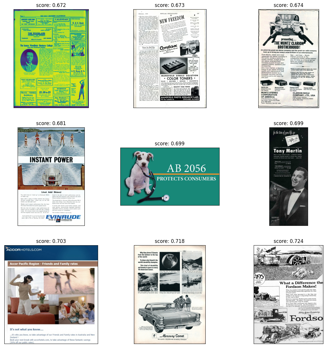
Now we can test the classifier with the open images dataset. We will start by looking at the misclassified images. This time it is the images that have the highest maximum score.

from PIL import Image
import numpy as np

non_advert_predictions = np.array(openimages_embedding_df.embedding.tolist()) @ linear_layer.T
non_advert_predictions = non_advert_predictions.max(axis=1)

print(f"overall accuracy of: {(non_advert_predictions <= 0).astype(float).sum() / len(openimages_embedding_df):0.3f}")
print(f"total misclassified: {(non_advert_predictions > 0).astype(int).sum():,} of {len(openimages_embedding_df):,}")

overall accuracy of: 0.949
total misclassified: 3,322 of 64,832

Code

scores = non_advert_predictions.argsort()[-9:]
show_image_block(
    openimages_embedding_df.iloc[scores].file,
    non_advert_predictions[scores],
    folder=OPENIMAGES_FOLDER,
)

Here we can see that the misclassified images are either adverts or strongly resemble adverts. Is this really a misclassification or is it a problem with the dataset?

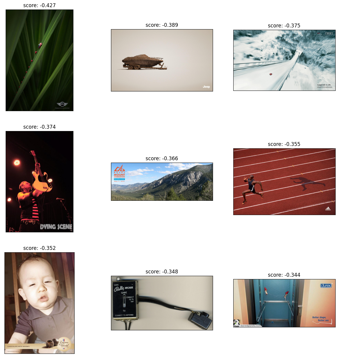
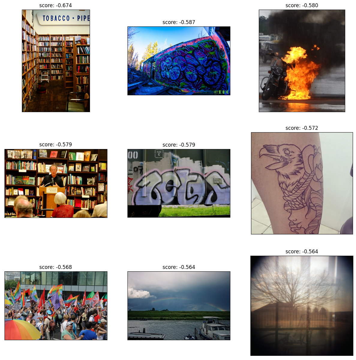
The next thing is to review the best classifications, those images with the lowest maximum score.

Code

scores = non_advert_predictions.argsort()[:9]
show_image_block(
    openimages_embedding_df.iloc[scores].file,
    non_advert_predictions[scores],
    folder=OPENIMAGES_FOLDER,
)

These images are not adverts and have some variation which is nice.

Broadly though there is clearly a problem with the open images dataset. It contains adverts. The dataset was sourced from the internet and I understood it to be primarily user generated content. It seems surprising to me that individuals would include adverts, but here we are.

While these overall results are slightly weaker than the test set suggested the evaluation seems solid. I’m happy with how this went.