Explainability Principles - Working In Reverse

I showed my recent model explainability work to a colleague. His response was interesting and I’m going to explore it in this post.

In my previous exploration of CLIP explainability I proposed the following principles:

• The composite value should be seen as the decomposition of the original value, that is \(V = \sum_{i = 0}^{n} C_i\).
• The individual entry in the composite output value should be related to the influence of the individual input value.

He is very good at mathematics and defined the overall principles in a more consistent way, and then used that to define an alternative derivation of \(C_i\). If the alternative approach results in different tracking numbers then the principles that I have proposed do not form a complete definition.

Mysterious Colleague Definition

Consider an arbitrary neural network which takes as input a tensor. Choose any “point” / place / position (whatever you want to call it) \(p\) in the network. \(p\) could be at the end of the network, e.g. a predicted class probability, or any intermediate point in the network. Denote by \(F_p(X)\) the function which maps the input tensor to the value calculated at point \(p\) in the network.

Now let’s take a particular input \(V\) where

\[ V = \sum_{i=1}^{N} C_i \]

i.e. \(V\) has been “split up” into \(N\) components \(C_1 \dots C_N\). We wish to understand how each component \(C_i\) contributes to the value \(F_p(V)\) which the network eventually computes.

For convenience let us write \(\bar{C_i}\) for the “complement” of the component \(C_i\) i.e. all of the rest of \(V\). Formally

\[ \bar{C_i} := V - C_i = \sum_{j \in \{1 \dots N\}, j \neq i} C_j \]

Suppose we run the netural network in turn on each \(\bar{C_i}\), as well as on the full input \(V\), and pick out the values that were computed at point \(p\) each time. This produces the values \(F_p(\bar{C_1}) \dots F_p(\bar{C_N})\) and also \(F_p(V)\). From there let’s compute

\[ D_i := F_p(V) - F_p(\bar{C_i}) \]

for each \(i \in \{i \dots N\}\). Let’s also compute an additional special value \(D_0\) as follows:

\[ D_0 := F_p(V) - \sum_{i=1}^{N} D_i \]

(This will turn out to be simply using the special extra component in the sum to “balance the books”.)

So what was the point of all that?

The point is that \(D_0, D_1 \dots D_N\) can actually serve as a “composite value” for the result \(F_p(V)\) at point \(p\) in the network. Why is that?

The first condition in your blog post is that “the composite value should be seen as the decomposition of the original value”. We can check this very simply as follows:

\[ \begin{aligned} \sum_{i=0}^{N} D_i &= D_0 + \sum_{i=1}^{N} D_i \\ &= F_p(V) - \sum_{i=1}^{N} D_i + \sum_{i=1}^{N} D_i \\ &= F_p(V) \end{aligned} \]

The second condition in your blog post is that “the individual entry in the composite output value should be related to the influence of the individual input value”. To see that this is the case we simply have to look at the definition of \(D_i\) (for \(i \neq 0\)) as

\[ \begin{aligned} D_i :=& \ F_p(V) - F_p(\bar{C_i}) \\ =& \ F_p(V) - \sum_{j \in \{1 \dots N\}, j \neq i} C_j \end{aligned} \]

This definition is saying exactly that \(D_i\) quantifies how much the output \(F_p(V)\) would change if \(C_i\) was dropped from the input.

So we have it! We just need to run the network \(N\) times, dropping each component of the input in turn, and collect up the results! :)

Empirical Validation

I really like this approach. The mathematical specification seems to be within my grasp and I can also use this to validate the calculation of the composite values. Talking to my colleague he said that if \(D_i\) does not match \(C_i\) from my original model then my mathematical principles are incomplete.

\(D_0\) in the definitions above is the bookkeeping factor, to make comparisons with the traced model from the previous post easier I am moving this to \(D_{N+1}\). Here I am going to run both the previous tracing model and the new proposed approach. Then the composite and overall output values can be compared.

Code

# from src/main/python/blog/tracing/v2023_02/layers.py
from typing import Optional, Tuple

import torch
from torch import nn
from transformers import CLIPModel
from transformers.models.clip.modeling_clip import (
    CLIPMLP,
    CLIPAttention,
    CLIPEncoder,
    CLIPEncoderLayer,
    CLIPVisionTransformer,
)


def load_tracing_image_model(
    model_name: str = "openai/clip-vit-base-patch32",
) -> CLIPModel:
    model = CLIPModel.from_pretrained(model_name)
    tracing_model = TracingCLIPVisionTransformer(
        model=model.vision_model, projection=model.visual_projection
    )
    tracing_model.eval()
    return tracing_model


class TracingCLIPVisionTransformer(nn.Module):
    def __init__(self, model: CLIPVisionTransformer, projection: nn.Linear) -> None:
        super().__init__()
        self.embeddings = model.embeddings
        # misspelling present in model
        self.pre_layernorm = TracingActivation(model.pre_layrnorm)
        self.encoder = CLIPEncoder(model.encoder.config)
        self.encoder.layers = nn.ModuleList(
            [TracingCLIPEncoderLayer(layer) for layer in model.encoder.layers]
        )
        self.post_layernorm = TracingActivation(model.post_layernorm)
        self.visual_projection = TracingLinear(projection)

    def forward(self, pixel_values: Optional[torch.Tensor] = None) -> torch.Tensor:
        embeddings = self.embeddings(pixel_values=pixel_values)
        _, image_regions, _ = embeddings.shape
        embeddings_traced = torch.zeros(
            *embeddings.shape, image_regions, device=embeddings.device
        )
        # 0 is the class embedding, that is not related to the image so it goes
        # in the constant index (last index)
        for i in range(image_regions - 1):
            embeddings_traced[:, i + 1, :, i] = embeddings[:, i + 1, :]
        embeddings_traced[:, 0, :, -1] = embeddings[:, 0, :]

        embeddings_normalized = self.pre_layernorm(embeddings_traced)
        encoded = self.encoder(
            inputs_embeds=embeddings_normalized,
            output_attentions=False,
            output_hidden_states=False,
            return_dict=False,
        )
        encoded = encoded[0]
        encoded = encoded[:, 0, :]
        encoded = self.post_layernorm(encoded)
        return self.visual_projection(encoded)


class TracingCLIPEncoderLayer(nn.Module):
    def __init__(self, layer: CLIPEncoderLayer) -> None:
        super().__init__()
        self.self_attn = TracingCLIPAttention(layer.self_attn)
        self.layer_norm1 = TracingActivation(layer.layer_norm1)
        self.mlp = TracingCLIPMLP(layer.mlp)
        self.layer_norm2 = TracingActivation(layer.layer_norm2)

    def forward(
        self,
        hidden_states: torch.Tensor,
        attention_mask: Optional[torch.Tensor],
        causal_attention_mask: Optional[torch.Tensor],
        output_attentions: bool,
    ) -> torch.Tensor:
        residual = hidden_states

        hidden_states = self.layer_norm1(hidden_states)
        hidden_states, attn_weights = self.self_attn(
            hidden_states=hidden_states,
            attention_mask=attention_mask,
            causal_attention_mask=causal_attention_mask,
            output_attentions=output_attentions,
        )
        hidden_states = residual + hidden_states

        residual = hidden_states
        hidden_states = self.layer_norm2(hidden_states)
        hidden_states = self.mlp(hidden_states)
        hidden_states = residual + hidden_states

        outputs = (hidden_states,)

        if output_attentions:
            outputs += (attn_weights,)

        return outputs


class TracingCLIPAttention(nn.Module):
    """Multi-headed attention from 'Attention Is All You Need' paper"""

    def __init__(self, layer: CLIPAttention) -> None:
        super().__init__()
        self.layer = layer

        self.k_proj = TracingLinear(layer.k_proj)
        self.v_proj = TracingLinear(layer.v_proj)
        self.q_proj = TracingLinear(layer.q_proj)
        self.out_proj = TracingLinear(layer.out_proj)
        self.bmm = TracingBMM()
        self.softmax = TracingActivation(nn.Softmax(dim=-1))

    def forward(
        self,
        hidden_states: torch.Tensor,
        attention_mask: Optional[torch.Tensor] = None,
        causal_attention_mask: Optional[torch.Tensor] = None,
        output_attentions: Optional[bool] = False,
    ) -> Tuple[torch.Tensor, Optional[torch.Tensor], Optional[Tuple[torch.Tensor]]]:
        """Input shape: Batch x Time x Channel x Tracing"""

        bsz, tgt_len, embed_dim, tracking_dim = hidden_states.size()

        # get query proj
        query_states = self.q_proj(hidden_states) * self.layer.scale
        key_states = self._shape(self.k_proj(hidden_states), -1, bsz, tracking_dim)
        value_states = self._shape(self.v_proj(hidden_states), -1, bsz, tracking_dim)

        proj_shape = (bsz * self.layer.num_heads, -1, self.layer.head_dim, tracking_dim)
        query_states = self._shape(query_states, tgt_len, bsz, tracking_dim).view(
            *proj_shape
        )
        key_states = key_states.view(*proj_shape)
        value_states = value_states.view(*proj_shape)

        src_len = key_states.size(1)
        attn_weights = self.bmm(query_states, key_states.transpose(1, 2))

        # code has been cut out here which relates to the
        # causal_attention_mask, attention_mask and error checking
        assert causal_attention_mask is None
        assert attention_mask is None

        attn_weights = self.softmax(attn_weights)

        if output_attentions:
            # this operation is a bit akward, but it's required to
            # make sure that attn_weights keeps its gradient.
            # In order to do so, attn_weights have to reshaped
            # twice and have to be reused in the following
            attn_weights_reshaped = attn_weights.view(
                bsz, self.layer.num_heads, tgt_len, src_len, tracking_dim
            )
            attn_weights = attn_weights_reshaped.view(
                bsz * self.layer.num_heads, tgt_len, src_len, tracking_dim
            )
        else:
            attn_weights_reshaped = None

        # this is not intended for training so dropout is removed entirely
        # attn_probs = nn.functional.dropout(attn_weights, p=self.dropout, training=self.training)
        attn_probs = attn_weights

        attn_output = self.bmm(attn_probs, value_states)
        attn_output = attn_output.view(
            bsz, self.layer.num_heads, tgt_len, self.layer.head_dim, tracking_dim
        )
        attn_output = attn_output.transpose(1, 2)
        attn_output = attn_output.reshape(bsz, tgt_len, embed_dim, tracking_dim)

        attn_output = self.out_proj(attn_output)

        return attn_output, attn_weights_reshaped

    def _shape(self, tensor: torch.Tensor, seq_len: int, bsz: int, tracking_dim: int):
        return (
            tensor.view(
                bsz, seq_len, self.layer.num_heads, self.layer.head_dim, tracking_dim
            )
            .transpose(1, 2)
            .contiguous()
        )


class TracingCLIPMLP(nn.Module):
    def __init__(self, layer: CLIPMLP) -> None:
        super().__init__()
        self.activation_fn = TracingActivation(layer.activation_fn)
        self.fc1 = TracingLinear(layer.fc1)
        self.fc2 = TracingLinear(layer.fc2)

    def forward(self, hidden_states: torch.Tensor) -> torch.Tensor:
        hidden_states = self.fc1(hidden_states)
        hidden_states = self.activation_fn(hidden_states)
        hidden_states = self.fc2(hidden_states)
        return hidden_states


class TracingLinear(nn.Module):
    def __init__(self, linear: nn.Linear) -> None:
        super().__init__()
        self.weight = linear.weight[:, :, None]
        self.bias = linear.bias

    def forward(self, xs: torch.Tensor) -> torch.Tensor:
        if len(xs.shape) == 3:
            mm = self._matrix_multiply_3d(xs)
        else:
            mm = self._matrix_multiply_4d(xs)
        if self.bias is not None:
            flat = mm.reshape(-1, *mm.shape[-2:])
            flat[:, :, -1] += self.bias
            mm = flat.reshape(*mm.shape)
        return mm

    def _matrix_multiply_3d(self, xs: torch.Tensor) -> torch.Tensor:
        return torch.einsum("bik,jik->bjk", xs, self.weight)

    def _matrix_multiply_4d(self, xs: torch.Tensor) -> torch.Tensor:
        return torch.einsum("Bbik,Bjik->Bbjk", xs, self.weight[None])


class TracingBMM(nn.Module):
    def forward(self, xs: torch.Tensor, ys: torch.Tensor) -> torch.Tensor:
        x_rollup = xs.sum(dim=-1).unsqueeze(-1)
        y_rollup = ys.sum(dim=-1).unsqueeze(-1)
        x_bmm = torch.einsum("bnmi,bmpi->bnpi", xs, y_rollup)
        y_bmm = torch.einsum("bnmi,bmpi->bnpi", x_rollup, ys)
        bmm = x_bmm + y_bmm
        bmm = bmm / 2
        return bmm


class TracingActivation(nn.Module):
    def __init__(self, activation_function: nn.Module) -> None:
        super().__init__()
        self.activation_function = activation_function

    def forward(self, composite_input_value: torch.Tensor) -> torch.Tensor:
        input_value = composite_input_value.sum(dim=-1)
        output_value = self.activation_function(input_value)

        # calculate the input magnitude and output magnitude for scaling each composite value set
        flat_composite_input_value = composite_input_value.reshape(
            -1, composite_input_value.shape[-1]
        )
        composite_input_magnitude = (
            flat_composite_input_value[:, :-1].abs().max(dim=-1)[0]
        )
        output_magnitude = output_value.abs().flatten()

        # calculate and apply the ratio
        ratio = output_magnitude / composite_input_magnitude
        flat_composite_output_value = flat_composite_input_value * ratio[:, None]
        # wipe out the values where the ratio would be nan, there is no input influence to track
        flat_composite_output_value[composite_input_magnitude == 0, :] = 0.0

        # check that the magnitude has been correctly scaled
        composite_output_magnitude = (
            flat_composite_output_value[:, :-1].abs().max(dim=-1)[0]
        )
        magnitude_difference = (composite_output_magnitude - output_magnitude).max()
        if magnitude_difference > 1e-5:
            raise AssertionError(f"magnitude check failed: {magnitude_difference:0.4g}")

        # use the unattributed constant value to ensure that the sum of the
        # composite value equals the original value
        composite_offset = flat_composite_output_value[:, :-1].sum(dim=-1)
        flat_composite_output_value[:, -1] = output_value.flatten() - composite_offset

        composite_output_value = flat_composite_output_value.reshape(
            composite_input_value.shape
        )
        return composite_output_value

Code

import warnings
from PIL import Image
import torch
from transformers import CLIPModel, CLIPProcessor

def preprocess_image(filename: str) -> torch.Tensor:
    image = Image.open(filename)
    processor = CLIPProcessor.from_pretrained("openai/clip-vit-base-patch32")
    with warnings.catch_warnings():
        # transformers/models/clip/processing_clip.py:142: FutureWarning:
        # `feature_extractor` is deprecated and will be removed in v5. Use `image_processor` instead.
        warnings.simplefilter("ignore")
        return processor.feature_extractor(image, return_tensors="pt").pixel_values


@torch.inference_mode()
def get_traced_output(pixel_values: torch.Tensor) -> torch.Tensor:
    model = load_tracing_image_model()
    model.eval()

    return model(pixel_values=pixel_values)

@torch.inference_mode()
def get_complement_output(pixel_values: torch.Tensor) -> torch.Tensor:
    model = CLIPModel.from_pretrained("openai/clip-vit-base-patch32")
    vision_model = model.vision_model
    model.eval()

    embeddings = vision_model.embeddings(pixel_values)
    embeddings = vision_model.pre_layrnorm(embeddings)
    region_count = embeddings.shape[1]

    # turn into complements and overall value
    # overall value is last one
    embeddings = embeddings.repeat(region_count + 1, 1, 1)

    # zero out inputs for each embedding to generate the complement input
    embeddings[range(region_count), range(region_count)] = 0.

    # calculate outputs
    encoder_outputs = vision_model.encoder(inputs_embeds=embeddings)
    last_hidden_state = encoder_outputs[0]
    pooled_output = last_hidden_state[:, 0, :]
    pooled_output = vision_model.post_layernorm(pooled_output)
    output = model.visual_projection(pooled_output)

    # current shape is batch x complement output
    # want to change this to embedding x composite output
    # C_i = V - \bar{C_i}
    V = output[-1]
    composite = V[:, None] - output[:-1].T

    # remember that the 0th embedding is the class embedding
    # we want to shift all the image region embeddings down by one
    composite[:, :-1] = composite[:, 1:].clone()

    # we don't need to retain the book-keeping value as we recalculate it here
    # C_{N+1} = V - sum C_i
    composite[:, -1] = V - composite[:, :-1].sum(dim=1)

    return composite

Code

import pandas as pd

pixel_values = preprocess_image("cat.jpg")
traced_output = get_traced_output(pixel_values)[0]
complement_output = get_complement_output(pixel_values)

composite_difference = traced_output - complement_output
value_difference = traced_output.sum(dim=1) - complement_output.sum(dim=1)

pd.DataFrame([
    {
        "label": "C_i difference",
        "max": composite_difference.max().item(),
        "mean": composite_difference.mean().item(),
        "min": composite_difference.min().item(),
    },
    {
        "label": "V difference",
        "max": value_difference.max().item(),
        "mean": value_difference.mean().item(),
        "min": value_difference.min().item(),
    },
])

	label	max	mean	min
0	C_i difference	32.786907	7.031485e-10	-42.984589
1	V difference	0.000010	2.789602e-08	-0.000008

We can see that the \(D_i\) values are quite different to \(C_i\) for the two approaches. The average difference is near zero, which is to be expected as the difference between the \(V\) values is very small. The book-keeping value ensures that the summed output will not vary from the original model output.

Complement Visualization

Given this the mathematical principles that I defined are incomplete or incorrect. Are the results of this complement approach better?

Code

import warnings

import pandas as pd
import torch
import torch.nn.functional as F
from transformers import CLIPModel, CLIPProcessor
from PIL import Image
from torchvision.transforms import ToPILImage
import matplotlib.pyplot as plt

def show_weights(traced_embedding: torch.Tensor, prompt: str) -> None:
    weights = get_weights(traced_embedding, prompt, show_similarity=True)
    show_region_attention(
        pixel_values,
        weights,
    )

def get_weights(traced_embedding: torch.Tensor, prompt: str, show_similarity: bool = False) -> torch.Tensor:
    text_embedding = get_text_embedding(prompt)
    text_embedding = text_embedding[0]

    if show_similarity:
        similarity = F.cosine_similarity(traced_embedding.sum(dim=-1), text_embedding, dim=0)
        print(f"cosine similarity: {similarity:0.4g}")

    weights = traced_embedding[:, :-1] * text_embedding[:, None]

    weights = weights.T.sum(dim=-1)
    weights = weights.sigmoid()
    weights = weights * 2 - 1
    weights = F.relu(weights)
    return weights

def get_similarity(traced_embedding: torch.Tensor, prompt: str) -> float:
    text_embedding = get_text_embedding(prompt)
    text_embedding = text_embedding[0]

    similarity = F.cosine_similarity(traced_embedding.sum(dim=-1), text_embedding, dim=0)
    return similarity.item()
    

@torch.inference_mode()
def get_text_embedding(prompt: str) -> torch.Tensor:
    processor = CLIPProcessor.from_pretrained("openai/clip-vit-base-patch32")
    model = CLIPModel.from_pretrained("openai/clip-vit-base-patch32")

    model.eval()

    text_features = processor.tokenizer([prompt], return_tensors="pt")
    text_outputs = model.text_model(**text_features)
    text_embeds = text_outputs[1] # pooler_output
    return model.text_projection(text_embeds)

image_mean = torch.tensor([
    0.48145466,
    0.4578275,
    0.40821073
])
image_std = torch.tensor([
    0.26862954,
    0.26130258,
    0.27577711
])

def show_region_attention(pixel_values: torch.Tensor, attention: torch.Tensor) -> None:
    # need to resize attention to match the values
    attention = attention.reshape(7, 7)
    attention = attention.to(float)
    attention = attention.repeat_interleave(32, dim=0).repeat_interleave(32, dim=1)
    # sigmoid means the values are already between 0 and 1
    # attention = attention - attention.min()
    # attention = attention / attention.max()
    
    pixel_values = pixel_values[0]
    pixel_values = (pixel_values * image_std[:, None, None]) + image_mean[:, None, None]
    scaled_values = pixel_values * attention

    fig, axes = plt.subplots(1,3, figsize=(224/10,224*3/10))
    axes[0].imshow(ToPILImage()(pixel_values))
    axes[1].imshow(ToPILImage()(scaled_values))
    axes[2].imshow(ToPILImage()(attention), cmap="binary_r")
    for axis in axes:
        axis.axis('off')

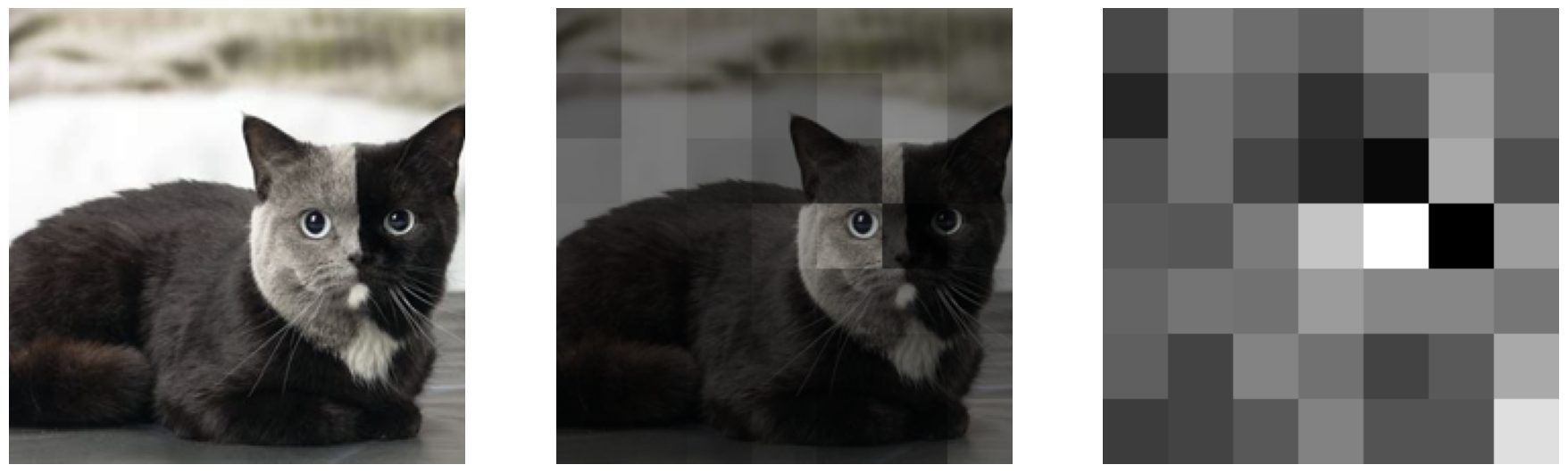
We can start by visualizing the approach from the previous post. I was quite pleased about how well it identified the face of the cat as an area that contributes to the classification.

show_weights(traced_output, "a rendering of a cat.")

cosine similarity: 0.2972

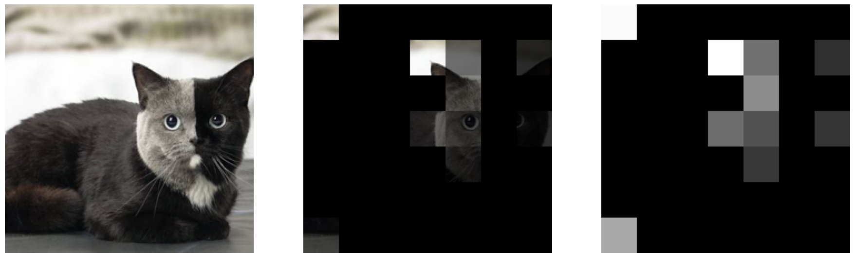
We can then compare this to the complement output. Does that identify particular areas of the image as contributing to the classification?

show_weights(complement_output, "a rendering of a cat.")

cosine similarity: 0.2971

The results of this are far less convincing. It has identified the eye as contributing strongly. Overall it suggests that the whole image contributes to the classification.

Quality Evaluation

Which approach is better?

We are trying to identify the parts of the image which contribute to the classification. If we take these weights and use them to reduce the embedding then which one causes it to lose catness fastest? Does this approach need some kind of scaling to accomodate the fact that the \(\bar{C_i}\) approach says that nearly the entire image contributes?

Code

prompt = "a rendering of a cat."
traced_weights = get_weights(traced_output, prompt)
complement_weights = get_weights(complement_output, prompt)

similarity = pd.Series({
    "traced": get_similarity(traced_output, prompt),
    "complement": get_similarity(complement_output, prompt),
})

pd.DataFrame({
    "average intensity": pd.Series({
        "traced": traced_weights.mean().item(),
        "complement": complement_weights.mean().item(),
    }),
    "cosine similarity": similarity,
})

	average intensity	cosine similarity
traced	0.101144	0.29715
complement	0.468777	0.29715

There are two ways that we can evaluate this - we can see how well the catness is retained when blanking out the other regions of the image, and we can see how quickly the catness is lost when blanking out the highlighted areas of the image.

The problem with the complement approach is that it has assigned some weight to the majority of the image. To fairly compare the two approaches we need to change the image by a similar amount using each method.

I’m going to solve this scaling issue by taking a target intensity of the image (0 = pure black, 1 = original image). Then the weights will be adjusted to achieve an intended image intensity. The same intensity should mean comparable results.

Code

import warnings

import torch
from transformers import CLIPModel, CLIPProcessor

model = CLIPModel.from_pretrained("openai/clip-vit-base-patch32")
prompt_embedding = get_text_embedding("a rendering of a cat.")[0]

def similiarity_pixel_values(
    pixel_values: torch.Tensor,
    weight: torch.Tensor,
    ratio: float,
) -> torch.Tensor:
    if weight.mean() < ratio:
        return np.nan
    output = use_weighted_pixel_values(
        pixel_values=pixel_values,
        weight=weight,
        ratio=ratio,
    )
    return F.cosine_similarity(
        output,
        prompt_embedding,
        dim=0,
    ).item()

def similiarity_embeddings(
    pixel_values: torch.Tensor,
    weight: torch.Tensor,
    ratio: float,
) -> torch.Tensor:
    if weight.mean() < ratio:
        return np.nan
    output = use_weighted_embeddings(
        pixel_values=pixel_values,
        weight=weight,
        ratio=ratio,
    )
    return F.cosine_similarity(
        output,
        prompt_embedding,
        dim=0,
    ).item()

@torch.inference_mode()
def use_weighted_pixel_values(
    pixel_values: torch.Tensor,
    weight: torch.Tensor,
    ratio: float,
) -> torch.Tensor:
    vision_model = model.vision_model
    model.eval()

    weight = scale_weight(weight, ratio)
    weight = weight.reshape(7, 7)
    weight = weight.repeat_interleave(32, dim=0).repeat_interleave(32, dim=1)
    pixel_values = pixel_values * weight[None, None]

    embeddings = vision_model.embeddings(pixel_values)
    embeddings = vision_model.pre_layrnorm(embeddings)

    # calculate outputs
    encoder_outputs = vision_model.encoder(inputs_embeds=embeddings)
    last_hidden_state = encoder_outputs[0]
    pooled_output = last_hidden_state[:, 0, :]
    pooled_output = vision_model.post_layernorm(pooled_output)
    return model.visual_projection(pooled_output)[0]

@torch.inference_mode()
def use_weighted_embeddings(
    pixel_values: torch.Tensor,
    weight: torch.Tensor,
    ratio: float,
) -> torch.Tensor:
    vision_model = model.vision_model
    model.eval()

    weight = scale_weight(weight, ratio)
    embeddings = vision_model.embeddings(pixel_values)
    embeddings = vision_model.pre_layrnorm(embeddings)
    embeddings[0, 1:] = embeddings[0, 1:] * weight[:, None]

    # calculate outputs
    encoder_outputs = vision_model.encoder(inputs_embeds=embeddings)
    last_hidden_state = encoder_outputs[0]
    pooled_output = last_hidden_state[:, 0, :]
    pooled_output = vision_model.post_layernorm(pooled_output)
    return model.visual_projection(pooled_output)[0]

def scale_weight(weight: torch.Tensor, ratio: float) -> torch.Tensor:
    # the aim here is to reduce the image by ratio amount
    # the weight will be adjusted such that it's mean is the ratio
    # if the weight average is less than the ratio then it cannot be applied
    weight_mean = weight.mean()
    if weight_mean < ratio:
        return torch.zeros_like(weight, device=weight.device)
    weight = weight * (ratio / weight_mean)
    return weight

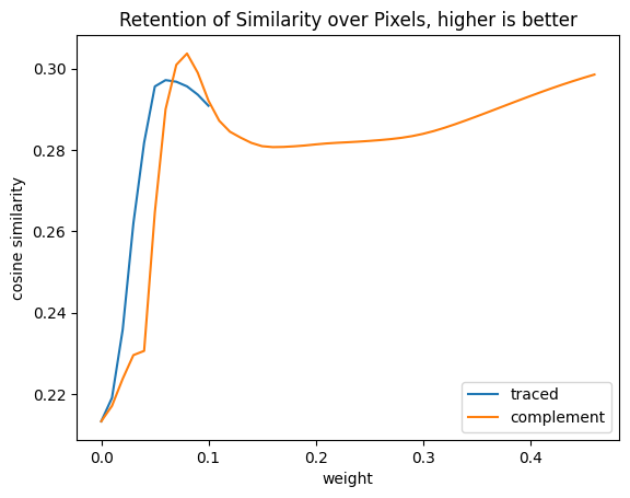
Retaining Only Cat

To start with we can test keeping the areas of the image that influence the cat classification, and removing the rest. If the assignment of influence is accurate then this should result in minimal loss of similarity. As more information is lost I would expect the similarity to decrease.

Code

import torch.nn.functional as F
import pandas as pd
import numpy as np

step = 0.01
df = pd.DataFrame([
    {
        "weight": ratio,
        "traced": similiarity_pixel_values(
            pixel_values,
            weight=traced_weights,
            ratio=ratio,
        ),
        "complement": similiarity_pixel_values(
            pixel_values,
            weight=complement_weights,
            ratio=ratio,
        ),
    }
    for ratio in np.arange(0, 1. + step, step)
])
df = df.set_index("weight")

df.plot(
    title="Retention of Similarity over Pixels, higher is better",
    ylabel="cosine similarity",
)

pd.DataFrame({
    "first cosine similarity": {
        "traced": df.traced.dropna().iloc[-1],
        "complement": df.complement.dropna().iloc[-1],
    },
    "highest cosine similarity": df.max(),
    "original cosine similarity": similarity,
})

	first cosine similarity	highest cosine similarity	original cosine similarity
traced	0.290884	0.297186	0.29715
complement	0.298550	0.303719	0.29715

Code

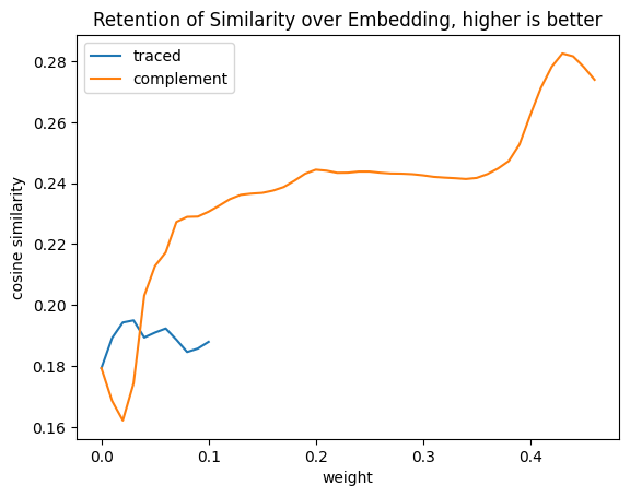
import torch.nn.functional as F
import pandas as pd
import numpy as np

step = 0.01
df = pd.DataFrame([
    {
        "weight": ratio,
        "traced": similiarity_embeddings(
            pixel_values,
            weight=traced_weights,
            ratio=ratio,
        ),
        "complement": similiarity_embeddings(
            pixel_values,
            weight=complement_weights,
            ratio=ratio,
        ),
    }
    for ratio in np.arange(0, 1+step, step)
])
df = df.set_index("weight")

df.plot(
    title="Retention of Similarity over Embedding, higher is better",
    ylabel="cosine similarity",
)

pd.DataFrame({
    "first cosine similarity": {
        "traced": df.traced.dropna().iloc[-1],
        "complement": df.complement.dropna().iloc[-1],
    },
    "highest cosine similarity": df.max(),
    "original cosine similarity": similarity,
})

	first cosine similarity	highest cosine similarity	original cosine similarity
traced	0.187947	0.194993	0.29715
complement	0.273914	0.282538	0.29715

These graphs are far from what I was expecting. I was hoping for a smoother reduction towards zero as the image lost information, and I was hoping that my original approach would at least retain more of the similarity for the same reduction of information. Both of these are not borne out by the data.

The alteration of the pixels to retain only what was considered important can actually boost the similarity beyond the original score. Then the reduction as the image is darkened is mostly flat. Thinking about this, a picture of a cat in a dark room is still visibly a cat, so the model is performing well over what amounts to a variation in lighting.

The alteration of the embeddings has far more unusual results. This time the traced alterations significantly impact the results and don’t really vary that much as they go to zero. Complement manages to match less before reaching absolute zero embeddings.

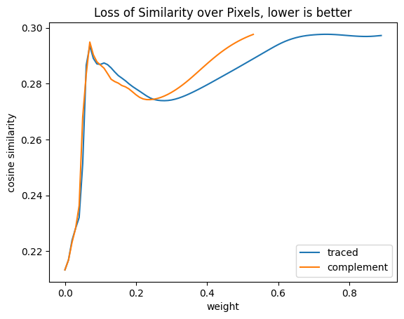
Removing Cat

Now we can test removing the areas of the image that influence the cat classification. I would expect this change to maximally reduce the cat classification. As more information is lost I would expect the similarity to continue to decrease.

Code

import torch.nn.functional as F
import pandas as pd
import numpy as np

inverse_traced_weights = 1 - traced_weights
inverse_complement_weights = 1 - complement_weights

step = 0.01
df = pd.DataFrame([
    {
        "weight": ratio,
        "traced": similiarity_pixel_values(
            pixel_values,
            weight=inverse_traced_weights,
            ratio=ratio,
        ),
        "complement": similiarity_pixel_values(
            pixel_values,
            weight=inverse_complement_weights,
            ratio=ratio,
        ),
    }
    for ratio in np.arange(0, 1+step, step)
])
df = df.set_index("weight")

df.plot(
    title="Loss of Similarity over Pixels, lower is better",
    ylabel="cosine similarity",
)

pd.DataFrame({
    "first cosine similarity": {
        "traced": df.traced.dropna().iloc[-1],
        "complement": df.complement.dropna().iloc[-1],
    },
    "highest cosine similarity": df.max(),
    "lowest cosine similarity": df.min(),
    "original cosine similarity": similarity,
})

	first cosine similarity	highest cosine similarity	lowest cosine similarity	original cosine similarity
traced	0.297202	0.297638	0.213328	0.29715
complement	0.297607	0.297607	0.213328	0.29715

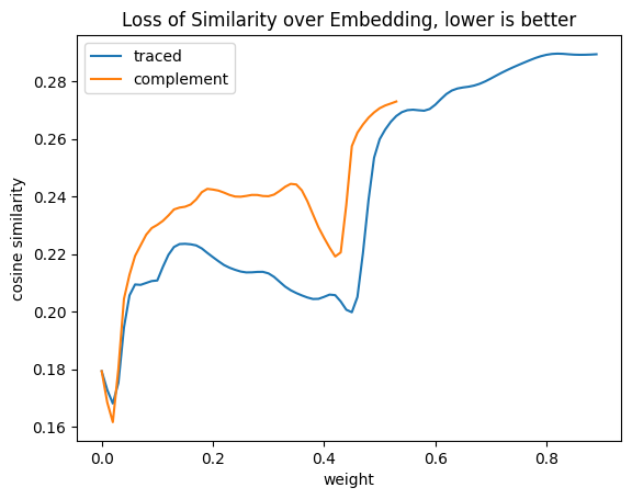
Code

import torch.nn.functional as F
import pandas as pd
import numpy as np

inverse_traced_weights = 1 - traced_weights
inverse_complement_weights = 1 - complement_weights

step = 0.01
df = pd.DataFrame([
    {
        "weight": ratio,
        "traced": similiarity_embeddings(
            pixel_values,
            weight=inverse_traced_weights,
            ratio=ratio,
        ),
        "complement": similiarity_embeddings(
            pixel_values,
            weight=inverse_complement_weights,
            ratio=ratio,
        ),
    }
    for ratio in np.arange(0, 1+step, step)
])
df = df.set_index("weight")

df.plot(
    title="Loss of Similarity over Embedding, lower is better",
    ylabel="cosine similarity",
)

pd.DataFrame({
    "first cosine similarity": {
        "traced": df.traced.dropna().iloc[-1],
        "complement": df.complement.dropna().iloc[-1],
    },
    "highest cosine similarity": df.max(),
    "lowest cosine similarity": df.min(),
    "original cosine similarity": similarity,
})

	first cosine similarity	highest cosine similarity	lowest cosine similarity	original cosine similarity
traced	0.289322	0.289534	0.168108	0.29715
complement	0.272930	0.272930	0.161632	0.29715

Again these images are not showing what I expected. The initial similarity after applying the filter is very similar to the original, indicating that removing the cat according to the relative influence had limited impact. After that the graph gets really strange, with both approaches showing a recovery of cat similarity after a dip.

Conclusions

I think that altering the embeddings is a poor way to judge the quality of the influence assignment. The embeddings incorporate image data, as well as bias from the convolutional layers and the positional embedding. A pure black image would still have non zero embeddings due to the bias and positional embedding. This means that scaling the embeddings down to zero produces inputs that the model would not experience during training.

When considering the pixels is the use of influence that was calculated over embeddings really going to work for the pixels that contributed to that? This should be the case as the convolutions do not pull from outside the 32x32 region and the bias and positional embedding are constant. The problem with the evaluation is that darkening the image does not significantly change the subject, and that is how the partial influence has been implemented, so interpreting the results is hard.

There are two evaluation approaches which could work with this. The first is to derive the change to the image which produces the greatest loss of a given classification. This makes sense because if this technique identifies the inputs that most influence the output, then changing those inputs should result in a large change in output.

The second is to identify the region of the image which contributes most to the classification and then compare that to some existing bounding box for the subject. Bounding box comparisons make sense as we would expect the cat classification to come from the cat within the image. This does rely on the model itself incorporating that behaviour.

Both of these approaches would be worth further investigation.