LLaMA

I’ve downloaded the weights for the Facebook LLaMA model (Touvron et al. 2023). This can be loaded using huggingface so I want to try it out (docs).

Touvron, Hugo, Thibaut Lavril, Gautier Izacard, Xavier Martinet, Marie-Anne Lachaux, Timothée Lacroix, Baptiste Rozière, et al. 2023. “LLaMA: Open and Efficient Foundation Language Models.” https://arxiv.org/abs/2302.13971.

The only problem is that the huggingface code has not made it into a release yet, and I don’t really want to build from source. I really rate their code so I’m going to download it to a local folder and add that to the sys path and that should let me load the llama model.

Convert Model Format

The weights are stored in a format which is not compatible with the huggingface implementation. We have to convert the weights to huggingface format. This is done by the transformers/models/llama/convert_llama_weights_to_hf.py script.

The script can be reviewed here (I’ve pinned that to the version I am using, it’s likely been updated since).

Code

from pathlib import Path
import sys

# transformers commit 559a45d1 2023-04-03 11:06:25
TRANSFORMERS_FOLDER = Path("/home/matthew/Programming/Python/transformers/src")

LLAMA_RAW = Path("/data/large-language-models/LLaMA")
LLAMA_HUGGINGFACE = Path("/data/large-language-models/LLaMA-huggingface")

if str(TRANSFORMERS_FOLDER) not in sys.path:
    sys.path.insert(0, str(TRANSFORMERS_FOLDER))

To keep everything within this notebook I am invoking the relevant methods directly.

Code

from pathlib import Path
from datetime import datetime

def convert_model(input_folder: Path, output_folder: Path, model_size: str) -> None:
    from transformers.models.llama.convert_llama_weights_to_hf import write_model, write_tokenizer

    tokenizer_file = input_folder / "tokenizer.model"
    model_folder = input_folder / model_size
    assert tokenizer_file.exists(), f"{tokenizer_file} not found"
    assert model_folder.exists(), f"{model_folder} not found"
    output_folder = output_folder / model_size
    
    model_start = datetime.now()
    write_model(
        model_path=output_folder,
        input_base_path=model_folder,
        model_size=model_size,
    )
    model_end = datetime.now()
    print(f"written model in {model_end-model_start}")

    tokenizer_start = datetime.now()
    write_tokenizer(
        tokenizer_path=output_folder,
        input_tokenizer_path=tokenizer_file,
    )
    tokenizer_end = datetime.now()
    print(f"written tokenizer in {tokenizer_end-tokenizer_start}")

convert_model(
    input_folder=LLAMA_RAW,
    output_folder=LLAMA_HUGGINGFACE,
    model_size="7B",
)

Code

convert_model(
    input_folder=LLAMA_RAW,
    output_folder=LLAMA_HUGGINGFACE,
    model_size="13B",
)

Fetching all parameters from the checkpoint at /data/large-language-models/LLaMA/13B.
Loading the checkpoint in a Llama model.

Saving in the Transformers format.
written model in 0:08:12.766689
Fetching the tokenizer from /data/large-language-models/LLaMA/tokenizer.model.
written tokenizer in 0:00:00.013171

Inspect Model

With the conversion out of the way it would be good to review the model to see how it compares to the smaller models that I am more familiar with.

Code

from transformers import LlamaForCausalLM, LlamaTokenizer

tokenizer = LlamaTokenizer.from_pretrained(LLAMA_HUGGINGFACE)
model = LlamaForCausalLM.from_pretrained(LLAMA_HUGGINGFACE)

Let’s start by reviewing text tokenization. I’m interested to see if it adds a start token as well as how it encodes specific words.

Code

word_to_id = tokenizer.get_vocab()
id_to_word = dict(zip(word_to_id.values(), word_to_id.keys()))

tokens = tokenizer(
    "hello worldle",
    return_tensors="pt",
).input_ids

for word, token in zip(
    tokenizer.batch_decode(tokens[0, :, None]),
    tokens[0].tolist(),
):
    print(f"{token} is '{word}' ({id_to_word[token]})")

1 is ' ' (<s>)
22172 is ' hello' (▁hello)
3186 is ' world' (▁world)
280 is ' le' (le)

This is interesting. There is the start token. I’m more interested in how the words are represented in the vocab, as the start of a word gets a special token prefix instead of the continuation.

We can also dig into the vocab slightly to see how the byte pair encoding is built up and if the model is multilingual.

Code

print("first 10 tokens")
for word, token in list(word_to_id.items())[:10]:
    print(f"{token} is {word}")

print("last 10 tokens")
for word, token in list(word_to_id.items())[-10:]:
    print(f"{token} is {word}")

first 10 tokens
0 is <unk>
1 is <s>
2 is </s>
3 is <0x00>
4 is <0x01>
5 is <0x02>
6 is <0x03>
7 is <0x04>
8 is <0x05>
9 is <0x06>
last 10 tokens
31990 is ὀ
31991 is げ
31992 is べ
31993 is 边
31994 is 还
31995 is 黃
31996 is 왕
31997 is 收
31998 is 弘
31999 is 给

It looks like the byte pair encoding is building up from raw bytes, and that the model is multilingual. Both are very encouraging. How does it handle emoji?

tokens = tokenizer(
    "😃💁",
    return_tensors="pt",
).input_ids

for word, token in zip(
    tokenizer.batch_decode(tokens[0, :, None]),
    tokens[0].tolist(),
):
    print(f"{token} is '{word}' ({id_to_word[token]})")

1 is ' ' (<s>)
29871 is ' ' (▁)
243 is ' �' (<0xF0>)
162 is ' �' (<0x9F>)
155 is ' �' (<0x98>)
134 is ' �' (<0x83>)
243 is ' �' (<0xF0>)
162 is ' �' (<0x9F>)
149 is ' �' (<0x92>)
132 is ' �' (<0x81>)

Ha, it really has just broken it down into individual bytes. It’s interesting that the word start token has such a large id.

What about the model stats? For reference bert base uncased accepts up to 512 tokens, has an internal embedding size of 768 and has 12 attention layers.

Code

model.config

LlamaConfig {
  "_name_or_path": "/data/large-language-models/LLaMA-7B-huggingface",
  "architectures": [
    "LlamaForCausalLM"
  ],
  "bos_token_id": 1,
  "eos_token_id": 2,
  "hidden_act": "silu",
  "hidden_size": 4096,
  "initializer_range": 0.02,
  "intermediate_size": 11008,
  "max_position_embeddings": 2048,
  "model_type": "llama",
  "num_attention_heads": 32,
  "num_hidden_layers": 32,
  "pad_token_id": 0,
  "rms_norm_eps": 1e-06,
  "tie_word_embeddings": false,
  "torch_dtype": "float16",
  "transformers_version": "4.28.0.dev0",
  "use_cache": true,
  "vocab_size": 32000
}

Here we can see that the model accepts up to 2,048 tokens, has an internal embedding size of 4,096 and has 32 attention layers. While this is much bigger than bert the input window pales in comparison to ChatGPT which accepts around 50k tokens. A larger input window allows for far more sophisticated prompts.

Text Generation

Now that we have made it through all of that, lets try generating some text. Since this has been loaded into the huggingface framework I can use the generate method that is available on every text model. A good description of the parameters that generate accepts is found here, I will try out each type of generation in turn.

The first is greedy generation which is the default. Let’s see how it deals with a very non specific input:

Code

def generate(input_text: str, **kwargs) -> str:
    tokens = tokenizer(
        input_text,
        return_tensors="pt",
        return_attention_mask=False,
    ).input_ids
    output = model.generate(tokens, **kwargs)
    return tokenizer.decode(output[0])

Code

%%time

print(
    generate("hello world", max_new_tokens=20)
)

 hello world! I'm a newbie here.
I'm a newbie here. I'
CPU times: user 2min 58s, sys: 0 ns, total: 2min 58s
Wall time: 17.9 s

It is quite quick considering that it is running on CPU. It generated 20 tokens in 17.9s which suggests around 900ms per token.

Obviously this output is very bad, managing to repeat itself extremely quickly. The next thing to test is the beam search. With 5 beams this should take around a minute and a half to complete.

Code

%%time

print(
    generate(
        "hello world",
        max_new_tokens=20,
        num_beams=5,
        early_stopping=True,
    )
)

 hello world
\end{code}

\begin{blockquote}

\begin{code}
CPU times: user 6min 30s, sys: 107 ms, total: 6min 30s
Wall time: 39.1 s

It seems that the model works well in parallel, as it’s cut around half the expected time off. The output now appears to be latex which is interesting but not really what I was looking for.

The problem with beam search is that it leads to very uninteresting output as it always picks the most likely composite output. When communicating the inclusion of unexpected words is a large part of how information is conveyed. The next methods use a random sampling of the output to encourage more variation.

We can start with pure sampling first:

Code

%%time

print(
    generate(
        "hello world",
        do_sample=True, 
        max_new_tokens=50, 
        top_k=0,
    )
)

 hello world! Welcome to my website where I cover a diverse amount of subjects with my non-binary perspective. Other Snarky Pseudonyms is the umbrella for whatever I may cover. Enjoy!
CPU times: user 6min 11s, sys: 19.3 ms, total: 6min 11s
Wall time: 37.1 s

This seems alright.

The huggingface blog post suggested that a pure sampling approach could have problems with selecting very unlikely words and losing coherence. To address this we can try altering the temperature. When the temperature is below 1 the probaility curve is sharper, making more probable words even more probable (and vice versa).

Code

%%time

print(
    generate(
        "hello world",
        do_sample=True,
        max_new_tokens=50,
        top_k=0,
        temperature=0.7,
    )
)

 hello world, welcome to my blog. my name is adrian and i live in denver colorado with my wonderful wife and two awesome kids. i'm a graphic designer, photographer, snowboarder, and cyclist. i have
CPU times: user 7min 10s, sys: 19.7 ms, total: 7min 10s
Wall time: 43 s

This is another fine utterance.

To wrap this up I’m now going to include both top-k and top-p sampling (top-k is the top-k most probable words, while top-p is the number of words that result in p probability mass).

Code

%%time

print(
    generate(
        "hello world",
        do_sample=True,
        max_new_tokens=50,
        top_k=50,
        top_p=0.95,
    )
)

 hello world – i see your data is safe with us and you have not to worry about it. you can relax and let the best data recovery software do their task. i am so happy that you find us as the best choice to do your data recovery.
CPU times: user 7min 10s, sys: 0 ns, total: 7min 10s
Wall time: 43 s

This sounds a bit like a scam email heh.

Given that the model can tokenize emoji, how does it handle generating text using them?

Code

%%time

print(
    generate(
        "😃💁🐻🌻🍔🍹",
        do_sample=True,
        max_new_tokens=50,
        top_k=50,
        top_p=0.95,
    )
)

 😃💁🐻🌻🍔🍹✌🏻👌💃😂💁🏻🐹🏋🏻🐾🌼���
CPU times: user 7min 13s, sys: 101 ms, total: 7min 13s
Wall time: 43.3 s

Prompted Task Completion

As a final evaluation can we provide the model with a prompt and some text to perform a task? I’m going to start with a conversational request to perform sentiment classification of a very clearly positive statement.

Code

%%time

print(
    generate(
        (
            "i love chatgpt it is the best ♥️💖💕💗💞💘\n\n"
            "Question: Does the preceding text express "
            "positive, negative or neutral sentiment:\n\n"
            "Answer: "
        ),
        do_sample=True,
        early_stopping=True,
        max_new_tokens=50,
        top_k=50,
        top_p=0.95,
    )
)

 i love chatgpt it is the best ♥️💖💕💗💞💘

Question: Does the preceding text express positive, negative or neutral sentiment:

Answer: 64% negative 36% positive

\begin{code}
def sentiment_analyze(text):
    sentiment = tf.contrib.text.sentiment.polarity_scores(text)
    polar
CPU times: user 7min 20s, sys: 288 ms, total: 7min 20s
Wall time: 44.1 s

That certainly is an interesting continuation. It also wants to generate some sentiment analysis code using tensorflow. Unfortunately I cannot find that module (tf.contrib itself is tensorflow v1 so it’s out of date).

In terms of classifying the text this has to be a failure.

When I did this kind of thing before I just inspected the next token that would be generated. Generation of text is expensive as it has to repeatedly run the model.

Let’s try that same utterance again but just look at the probability of positive, negative and neutral.

Code

positive_id = word_to_id["▁positive"]
neutral_id = word_to_id["▁neutral"]
negative_id = word_to_id["▁negative"]

Code

import torch
import pandas as pd

def sentiment(text: str) -> None:
    with torch.inference_mode():
        tokens = tokenizer(text, return_tensors="pt")
        output = model(**tokens)
        predictions = output.logits[0, -1, [positive_id, neutral_id, negative_id]]

    probabilities = dict(zip(
        ["positive", "neutral", "negative"],
        predictions.softmax(0).tolist()
    ))
    print(probabilities)

sentiment(
    (
        "i love chatgpt it is the best ♥️💖💕💗💞💘\n\n"
        "Question: Does the preceding text express "
        "positive, negative or neutral sentiment:\n\n"
        "Answer: "
    )
)

{'positive': 0.6832154989242554, 'neutral': 0.12581485509872437, 'negative': 0.19096963107585907}

This is way better.

Can we get more information using this next token approach? How about describing a word within the utterance? How does the per token probability vary across the vocabulary?

Code

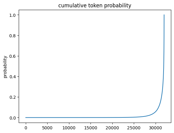
import torch
import pandas as pd

def show_next_token_probability(text: str) -> None:
    with torch.inference_mode():
        tokens = tokenizer(text, return_tensors="pt")
        output = model(**tokens)
        predictions = output.logits[0, -1]

    probabilities = predictions.softmax(0)
    sorted_tokens = probabilities.argsort(descending=False)
    probabilities = probabilities[sorted_tokens]
    pd.Series(probabilities.cumsum(0).numpy()).plot(
        title="cumulative token probability",
        ylabel="probability",
    )

    print(f"predicted next word for '{text}'")
    top_tokens = list(zip(
        tokenizer.batch_decode(sorted_tokens[-10:, None]),
        probabilities[-10:].tolist()
    ))[::-1]
    for word, probability in top_tokens:
        print(f"{word: >10}: {probability:0.4f}")

show_next_token_probability("I broke my apple today. apple is a")

predicted next word for 'I broke my apple today. apple is a'
      very: 0.0254
     brand: 0.0210
   company: 0.0191
  computer: 0.0180
          : 0.0176
      good: 0.0163
     small: 0.0156
     great: 0.0123
       big: 0.0120
       new: 0.0111

Here it is describing the word apple as a brand, company and computer. These results are interesting as this utterance is clearly (to me) about an iphone. So the LLaMA model can be used to perform some kind of entity disambiguation.

The cumulative token probability is very sharp, however it appears that at least 5,000 tokens have some probability mass even after softmax. How does that look before softmax?

Code

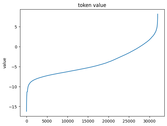
import torch
import pandas as pd

def show_next_token_value(text: str) -> None:
    with torch.inference_mode():
        tokens = tokenizer(text, return_tensors="pt")
        output = model(**tokens)
        predictions = output.logits[0, -1]

    sorted_tokens = predictions.argsort(descending=False)
    predictions = predictions[sorted_tokens]
    pd.Series(predictions.numpy()).plot(title="token value", ylabel="value")

show_next_token_value("I broke my apple today. apple is a")

It looks like the softmax roughly cut off the values at around 0. This distribution is far more flat than I would’ve expected. When I’ve previously worked with models they have been far more confident about the next token.

How does this compare to the embedding prior to the language model head?

Code

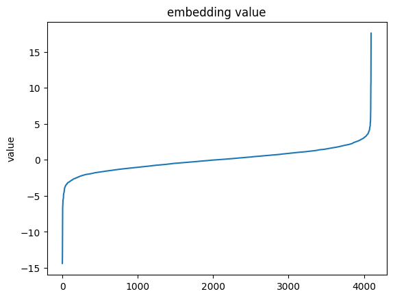
import torch
import pandas as pd

def show_next_embedding(text: str) -> None:
    with torch.inference_mode():
        tokens = tokenizer(text, return_tensors="pt")
        output = model.model(**tokens)
        predictions = output.last_hidden_state[0, -1]

    sorted_tokens = predictions.argsort(descending=False)
    predictions = predictions[sorted_tokens]
    pd.Series(predictions.numpy()).plot(title="embedding value", ylabel="value")

show_next_embedding("I broke my apple today. apple is a")

This is even more polarized! Most of the values cluster around zero while a very small number are highly positive or negative.

I had previously thought that the embedding prior to the language modelling head would be a better representation of the information inherent in the sentence, however that does not appear to be the case. The language modelling head itself may well point to the reason - it’s a simple linear layer. Language modelling has clearly moved within the model body so extracting a more semantic embedding from the model might be a case of sampling earlier or of retraining.

The very end of the model looks like this:

...
        (input_layernorm): LlamaRMSNorm()
        (post_attention_layernorm): LlamaRMSNorm()
      )
      (31): LlamaDecoderLayer(
        (self_attn): LlamaAttention(
          (q_proj): Linear(in_features=4096, out_features=4096, bias=False)
          (k_proj): Linear(in_features=4096, out_features=4096, bias=False)
          (v_proj): Linear(in_features=4096, out_features=4096, bias=False)
          (o_proj): Linear(in_features=4096, out_features=4096, bias=False)
          (rotary_emb): LlamaRotaryEmbedding()
        )
        (mlp): LlamaMLP(
          (gate_proj): Linear(in_features=4096, out_features=11008, bias=False)
          (down_proj): Linear(in_features=11008, out_features=4096, bias=False)
          (up_proj): Linear(in_features=4096, out_features=11008, bias=False)
          (act_fn): SiLUActivation()
        )
        (input_layernorm): LlamaRMSNorm()
        (post_attention_layernorm): LlamaRMSNorm()
      )
    )
    (norm): LlamaRMSNorm()
  )
  (lm_head): Linear(in_features=4096, out_features=32000, bias=False)
)

So the norm and lm_head are the only parts that really differ from the repeated attention layers.