Matthew’s Blog - Low Rank Adaptation (LoRA)

Low Rank Adaptation (Hu et al. 2021) is a technique for training large language models. It was originally evaluated against RoBERTa and GPT2 so it works on more moderate language models as well.

Hu, Edward J., Yelong Shen, Phillip Wallis, Zeyuan Allen-Zhu, Yuanzhi Li, Shean Wang, Lu Wang, and Weizhu Chen. 2021. “LoRA: Low-Rank Adaptation of Large Language Models.” https://arxiv.org/abs/2106.09685.

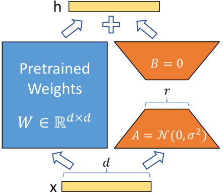
The aim of the technique is to fine tune an existing language model with only a small memory overhead. It works by creating a delta over the original weights. This delta is low memory because it is two matricies, \(A \in ℝ^{x \times r}\) and \(B \in ℝ^{r \times y}\), which exist for each target set of weights \(W \in ℝ^{x \times y}\). Memory is saved because the hyperparameter \(r\) is chosen such that the two matricies are significantly smaller than the original.

The training of the model is only allowed to alter the two matricies, \(A\) and \(B\). They are applied to the underlying weights \(W\) to produce the trained parameter \(W_t = W + AB\).

This is visualized in the original paper:

Example LoRA Layer

To start with we should define a single layer that has this technique applied. The linear layer is used in attention to alter the various inputs to the matrix multiplications, and so that is a good layer to alter.

Code

from torch import nn
import torch.nn.functional as F
import torch

class LoraLinear(nn.Module):
    def __init__(self, linear: nn.Linear, r: int, alpha: float) -> None:
        super().__init__()
        self.weight = nn.Parameter(linear.weight.data, requires_grad=False)
        if linear.bias is not None:
            self.bias = nn.Parameter(linear.bias.data, requires_grad=False)
        else:
            self.bias = None

        # Initialization from the paper, section 7.1
        x, y = linear.weight.shape
        self.a = nn.Parameter(torch.normal(0, 1, (x,r)) * (alpha / r))
        self.b = nn.Parameter(torch.zeros(r,y))

    def forward(self, x: torch.Tensor) -> torch.Tensor:
        wd = (self.a @ self.b) + self.weight
        return F.linear(x, wd, self.bias)

Given that the paper initializes \(B\) as zero we can check that this works by directly comparing outputs:

from torch import nn
import torch

base = nn.Linear(in_features=3, out_features=4, bias=True)
lora = LoraLinear(base, r=1, alpha=1)

with torch.inference_mode():
    x = torch.normal(0,1,(3,3))
    y_base = base(x)
    y_lora = lora(x)

(y_base - y_lora).abs().max()

tensor(0.)

We want to ensure that the optimizer will only alter \(A\) and \(B\). Let’s check that it does so. We can do that by training it with random data to see what the optimizer will alter.

Code

from torch import optim
import pandas as pd

lora = LoraLinear(base, r=1, alpha=1)
original = {
    name: parameter.data.clone().detach()
    for name, parameter in lora.named_parameters()
}

# apply optimizer to alter trainable parameters
# this is done twice as B starts at zero,
# so it needs an update before A can change
optimizer = optim.SGD(lora.parameters(), lr=0.1)
for _ in range(2):
    optimizer.zero_grad()
    x = torch.normal(0,1,(3,3))
    loss = lora(x)
    loss = loss ** 2
    loss = loss.sum()
    loss.backward() 
    optimizer.step()

updated = {
    name: parameter.data.clone().detach()
    for name, parameter in lora.named_parameters()
}

pd.DataFrame([
    {
        "name": name,
        "difference":
            (original[name] - updated[name])
                .abs()
                .max()
                .item(),
    }
    for name in original
])

	name	difference
0	weight	0.000000
1	bias	0.000000
2	a	0.602379
3	b	0.594993

This confirms that the optimizer is limited to the \(A\) and \(B\) matricies.

Train BERT using LoRA

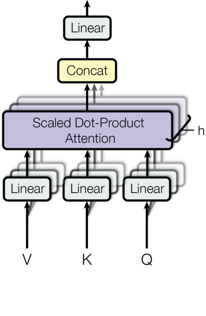
With this linear layer we can alter a transformer model to fine tune it. The linear layers in the attention block (Vaswani et al. 2017) were the original target for the fine tuning in the LoRA paper.

Vaswani, Ashish, Noam Shazeer, Niki Parmar, Jakob Uszkoreit, Llion Jones, Aidan N. Gomez, Lukasz Kaiser, and Illia Polosukhin. 2017. “Attention Is All You Need.” https://arxiv.org/abs/1706.03762.

Since I want to fine tune an existing model I am keen to take a language model and then fine tune it on a simple task like sentiment. This will involve replacing the original head with a classification one. As the replacement head will be untrained, I will zero out the weights for that.

Code

from pathlib import Path

MODEL_NAME = "bert-base-uncased"
BATCH_SIZE = 32

MODEL_RUN_FOLDER = Path("/data/blog/2023/05/17/low-rank-adaptation/runs")
MODEL_RUN_FOLDER.mkdir(parents=True, exist_ok=True)

Code

from transformers import AutoModelForSequenceClassification, AutoTokenizer
import logging

def load_lora_model(
    name: str,
    r: int,
    alpha: float,
    zero_head: bool = True,
) -> AutoModelForSequenceClassification:
    """
    This iterates through the model finding all linear layers,
    replacing them with the LoRA equivalent.
    """
    model = AutoModelForSequenceClassification.from_pretrained(name)

    for parameter in model.parameters():
        parameter.requires_grad = False

    # zero out the classification head
    # this code is specific to the model type!
    if zero_head:
        model.classifier.weight *= 0.
        model.classifier.bias *= 0.
    
    # since they have to be replaced in the parent,
    # this iterates through the modules
    # and then the children of those modules
    for module in model.modules():
        for attr, child in module.named_children():
            if not isinstance(child, nn.Linear):
                continue
            setattr(module, attr, LoraLinear(linear=child, r=r, alpha=alpha))
    return model


# disable warnings about uninitialized parameters
logging.getLogger("transformers.modeling_utils").setLevel(logging.ERROR)

base_model = AutoModelForSequenceClassification.from_pretrained(MODEL_NAME)
lora_model = load_lora_model(MODEL_NAME, r=1, alpha=1)
tokenizer = AutoTokenizer.from_pretrained(MODEL_NAME)

We can now try a limited train over this. I’ve loaded the same model without alteration in order to compare the LoRA train to a fine tune.

Code

import evaluate
from datasets import load_dataset
from transformers import EvalPrediction

def sst2_metric_simple(results: EvalPrediction) -> dict[str, float]:
    # convert raw model output into predicted class
    predictions = results.predictions.argmax(axis=1)
    targets = results.label_ids
    accuracy = (predictions == targets).mean().item()
    return {"accuracy": accuracy}

def encode(row: dict) -> list[int]:
    return tokenizer(
        row["sentence"],
        return_attention_mask=False,
        return_token_type_ids=False
    )

sst2_ds = load_dataset("glue", "sst2")
encoded_sst2_ds = sst2_ds.map(encode)

Found cached dataset glue (/home/matthew/.cache/huggingface/datasets/glue/sst2/1.0.0/dacbe3125aa31d7f70367a07a8a9e72a5a0bfeb5fc42e75c9db75b96da6053ad)

Loading cached processed dataset at /home/matthew/.cache/huggingface/datasets/glue/sst2/1.0.0/dacbe3125aa31d7f70367a07a8a9e72a5a0bfeb5fc42e75c9db75b96da6053ad/cache-1e7a3c4176f28664.arrow
Loading cached processed dataset at /home/matthew/.cache/huggingface/datasets/glue/sst2/1.0.0/dacbe3125aa31d7f70367a07a8a9e72a5a0bfeb5fc42e75c9db75b96da6053ad/cache-158aea0f60f8ead6.arrow
Loading cached processed dataset at /home/matthew/.cache/huggingface/datasets/glue/sst2/1.0.0/dacbe3125aa31d7f70367a07a8a9e72a5a0bfeb5fc42e75c9db75b96da6053ad/cache-0b773fb0bc2f6de3.arrow

Fine Tuning

We can establish a baseline for this sentiment analysis task by fine tuning the model. This is done without using the LoRA technique.

Code

from transformers import Trainer, TrainingArguments

training_args = TrainingArguments(
    per_device_train_batch_size=BATCH_SIZE,
    per_device_eval_batch_size=BATCH_SIZE,
    learning_rate=5e-5,
    warmup_ratio=0.06,
    optim="adamw_torch",

    report_to=[], # you'd use wandb for weights and biases

    evaluation_strategy="steps",
    max_steps=1_000,
    logging_steps=100,
    eval_steps=100,
    save_steps=100,

    load_best_model_at_end=True,
    metric_for_best_model="accuracy",
    greater_is_better=True,
    
    no_cuda=False,

    # output_dir is compulsory
    logging_dir=MODEL_RUN_FOLDER / "output",
    output_dir=MODEL_RUN_FOLDER / "output",
    overwrite_output_dir=True,
)

trainer = Trainer(
    model=base_model,
    args=training_args,
    train_dataset=encoded_sst2_ds["train"],
    eval_dataset=encoded_sst2_ds["validation"],
    tokenizer=tokenizer,
    compute_metrics=sst2_metric_simple,
)

trainer.train()

You're using a BertTokenizerFast tokenizer. Please note that with a fast tokenizer, using the `__call__` method is faster than using a method to encode the text followed by a call to the `pad` method to get a padded encoding.

[1000/1000 01:42, Epoch 0/1]

Step	Training Loss	Validation Loss	Accuracy
100	0.472400	0.296161	0.878440
200	0.303400	0.252073	0.905963
300	0.268700	0.307821	0.891055
400	0.233700	0.237452	0.907110
500	0.226800	0.221912	0.919725
600	0.205200	0.239878	0.903670
700	0.205700	0.213245	0.912844
800	0.203400	0.202326	0.919725
900	0.188600	0.201419	0.915138
1000	0.173500	0.206102	0.919725

TrainOutput(global_step=1000, training_loss=0.24812209510803224, metrics={'train_runtime': 102.6206, 'train_samples_per_second': 311.828, 'train_steps_per_second': 9.745, 'total_flos': 659093193676800.0, 'train_loss': 0.24812209510803224, 'epoch': 0.48})

A best accuracy of around 0.92 is pretty good.

LoRA Train

Now we can compare the LoRA train. The final layer of the model has not been trained and instead has been set to zero, so that will be a problem for this technique. If the LoRA modification is best against a tuned model then this will impact the accuracy.

Code

from transformers import Trainer, TrainingArguments

training_args = TrainingArguments(
    per_device_train_batch_size=BATCH_SIZE,
    per_device_eval_batch_size=BATCH_SIZE,
    learning_rate=5e-5,
    warmup_ratio=0.06,
    optim="adamw_torch",

    report_to=[], # you'd use wandb for weights and biases

    evaluation_strategy="steps",
    max_steps=1_000,
    logging_steps=100,
    eval_steps=100,
    save_steps=100,

    load_best_model_at_end=True,
    metric_for_best_model="accuracy",
    greater_is_better=True,
    
    no_cuda=False,

    # output_dir is compulsory
    logging_dir=MODEL_RUN_FOLDER / "output",
    output_dir=MODEL_RUN_FOLDER / "output",
    overwrite_output_dir=True,
)

trainer = Trainer(
    model=lora_model,
    args=training_args,
    train_dataset=encoded_sst2_ds["train"],
    eval_dataset=encoded_sst2_ds["validation"],
    tokenizer=tokenizer,
    compute_metrics=sst2_metric_simple,
)

trainer.train()

[1000/1000 01:55, Epoch 0/1]

Step	Training Loss	Validation Loss	Accuracy
100	0.677600	0.627938	0.595183
200	0.462500	0.364696	0.854358
300	0.360400	0.361056	0.854358
400	0.330500	0.330100	0.862385
500	0.342500	0.352120	0.850917
600	0.311300	0.340034	0.858945
700	0.337000	0.310727	0.864679
800	0.319600	0.297864	0.881881
900	0.314200	0.302110	0.871560
1000	0.300800	0.304568	0.868119

TrainOutput(global_step=1000, training_loss=0.37564347839355466, metrics={'train_runtime': 115.719, 'train_samples_per_second': 276.532, 'train_steps_per_second': 8.642, 'total_flos': 660387507056640.0, 'train_loss': 0.37564347839355466, 'epoch': 0.48})

The accuracy has reached 0.88 which is worse than the fine tune by 0.04. It would be good to check that the model has not trained the wrong weights to confirm that the training technique was correctly applied.

Code

from transformers import AutoModelForSequenceClassification, AutoTokenizer
import logging
import pandas as pd

# disable warnings about uninitialized parameters
logging.getLogger("transformers.modeling_utils").setLevel(logging.ERROR)

comparison_model = AutoModelForSequenceClassification.from_pretrained(MODEL_NAME)
comparison_model.to(lora_model.device)

# the classifier head in the LoRA model has been set to zero
comparison_model.classifier.weight.data *= 0.
comparison_model.classifier.bias.data *= 0.

lora_parameters = dict(lora_model.named_parameters())

difference_df = pd.DataFrame([
    {
        "name": name,
        "difference": 
            (parameter - lora_parameters[name])
                .abs()
                .max()
                .item(),
    }
    for name, parameter in comparison_model.named_parameters()
])
difference_df.difference.describe().to_frame()

	difference
count	201.0
mean	0.0
std	0.0
min	0.0
25%	0.0
50%	0.0
75%	0.0
max	0.0

Given that every difference to the original bert-base-uncased model is zero we can be sure that the improvement in accuracy is down to the training.

How do the parameter counts differ for these two models? As we can be sure that the training of the lora model is restricted to those parameters that we have added, we can just count the difference in size between the two models.

Code

from transformers import AutoModelForSequenceClassification
from torch import nn
import pandas as pd

def parameter_count(model: nn.Module) -> int:
    return sum(param.numel() for param in model.parameters())

bert_count = parameter_count(
    AutoModelForSequenceClassification.from_pretrained(MODEL_NAME)
)
lora_count = parameter_count(
    load_lora_model(MODEL_NAME, r=1, alpha=1)
)
lora_trainable_count = lora_count - bert_count

print(f"{MODEL_NAME} has {bert_count:,} trainable parameters")
print(f"{MODEL_NAME}-LoRA has {lora_trainable_count:,} trainable parameters")
print(f"The LoRA model has {lora_trainable_count * 100 / bert_count:0.3f}% of the trainable parameters")

bert-base-uncased has 109,483,778 trainable parameters
bert-base-uncased-LoRA has 168,194 trainable parameters
The LoRA model has 0.154% of the trainable parameters

Using only a rank 1 model we were able to get 0.88 accuracy against a 0.92 for a full train. This was achieved with just 0.15% of the trainable parameters. I can see why LoRA is so good for low resource training.

Finetuned Classifier Head

The LoRA technique was performed with the pretrained body but zero weights for the head. If we fine tune the head then how does the LoRA technique compare to the full fine tuning?

Code

from transformers import Trainer, TrainingArguments
from transformers import AutoModelForSequenceClassification, AutoTokenizer
import logging
from torch import optim

# disable warnings about uninitialized parameters
logging.getLogger("transformers.modeling_utils").setLevel(logging.ERROR)

finetuned_model = AutoModelForSequenceClassification.from_pretrained(MODEL_NAME)
tokenizer = AutoTokenizer.from_pretrained(MODEL_NAME)
optimizer = optim.Adam(finetuned_model.classifier.parameters(), lr=5e-5)

training_args = TrainingArguments(
    per_device_train_batch_size=BATCH_SIZE,
    per_device_eval_batch_size=BATCH_SIZE,
    learning_rate=5e-5,
    warmup_ratio=0.06,
    optim="adamw_torch",

    report_to=[], # you'd use wandb for weights and biases

    evaluation_strategy="steps",
    max_steps=1_000,
    logging_steps=100,
    eval_steps=100,
    save_steps=100,

    load_best_model_at_end=True,
    metric_for_best_model="accuracy",
    greater_is_better=True,
    
    no_cuda=False,

    # output_dir is compulsory
    logging_dir=MODEL_RUN_FOLDER / "output",
    output_dir=MODEL_RUN_FOLDER / "output",
    overwrite_output_dir=True,
)

trainer = Trainer(
    model=finetuned_model,
    args=training_args,
    train_dataset=encoded_sst2_ds["train"],
    eval_dataset=encoded_sst2_ds["validation"],
    tokenizer=tokenizer,
    compute_metrics=sst2_metric_simple,
    optimizers=(optimizer, None),
)

trainer.train()

finetuned_model.save_pretrained(MODEL_RUN_FOLDER / "finetuned")

You're using a BertTokenizerFast tokenizer. Please note that with a fast tokenizer, using the `__call__` method is faster than using a method to encode the text followed by a call to the `pad` method to get a padded encoding.

[1000/1000 01:38, Epoch 0/1]

Step	Training Loss	Validation Loss	Accuracy
100	0.691600	0.694776	0.503440
200	0.690100	0.691753	0.505734
300	0.686200	0.692615	0.510321
400	0.686600	0.684969	0.518349
500	0.684800	0.680387	0.535550
600	0.678100	0.683288	0.512615
700	0.677400	0.681707	0.511468
800	0.672600	0.680154	0.513761
900	0.675800	0.677699	0.522936
1000	0.675100	0.677616	0.521789

The accuracy has barely changed as this is only able to train the final layer. Once again we can check that the parameters have not changed.

Code

from transformers import AutoModelForSequenceClassification, AutoTokenizer
import logging
import pandas as pd

# disable warnings about uninitialized parameters
logging.getLogger("transformers.modeling_utils").setLevel(logging.ERROR)

finetuned_parameters = {
    name: parameter
    for name, parameter in finetuned_model.named_parameters()
}

pd.DataFrame([
    {
        "name": name,
        "difference": 
            (parameter - finetuned_parameters[name])
                .abs()
                .max()
                .item(),
    }
    for name, parameter in comparison_model.named_parameters()
])

	name	difference
0	bert.embeddings.word_embeddings.weight	0.000000
1	bert.embeddings.position_embeddings.weight	0.000000
2	bert.embeddings.token_type_embeddings.weight	0.000000
3	bert.embeddings.LayerNorm.weight	0.000000
4	bert.embeddings.LayerNorm.bias	0.000000
...	...	...
196	bert.encoder.layer.11.output.LayerNorm.bias	0.000000
197	bert.pooler.dense.weight	0.000000
198	bert.pooler.dense.bias	0.000000
199	classifier.weight	0.066472
200	classifier.bias	0.000405

201 rows × 2 columns

With this we can now try training the lora model again.

Fine Tuning the Finetuned Classifier Head

We can try further fine tuning the entire model to see how much difference it makes. This is a nice excersize as it is the normal way of training such a model. If you fine tune the whole model when the classification head is randomly initialized then the poor performance of the head can degrade the model with irrelevant updates before it becomes suitably good.

So training just the classification head improves it so that updates to the whole model are high quality. Let’s see how much the performance differs.

Code

from transformers import Trainer, TrainingArguments
from transformers import AutoModelForSequenceClassification, AutoTokenizer

base_model = AutoModelForSequenceClassification.from_pretrained(
    MODEL_RUN_FOLDER / "finetuned"
)
tokenizer = AutoTokenizer.from_pretrained(MODEL_NAME)

training_args = TrainingArguments(
    per_device_train_batch_size=BATCH_SIZE,
    per_device_eval_batch_size=BATCH_SIZE,
    learning_rate=5e-5,
    warmup_ratio=0.06,
    optim="adamw_torch",

    report_to=[], # you'd use wandb for weights and biases

    evaluation_strategy="steps",
    max_steps=1_000,
    logging_steps=100,
    eval_steps=100,
    save_steps=100,

    load_best_model_at_end=True,
    metric_for_best_model="accuracy",
    greater_is_better=True,
    
    no_cuda=False,

    # output_dir is compulsory
    logging_dir=MODEL_RUN_FOLDER / "output",
    output_dir=MODEL_RUN_FOLDER / "output",
    overwrite_output_dir=True,
)

trainer = Trainer(
    model=base_model,
    args=training_args,
    train_dataset=encoded_sst2_ds["train"],
    eval_dataset=encoded_sst2_ds["validation"],
    tokenizer=tokenizer,
    compute_metrics=sst2_metric_simple,
)

trainer.train()

You're using a BertTokenizerFast tokenizer. Please note that with a fast tokenizer, using the `__call__` method is faster than using a method to encode the text followed by a call to the `pad` method to get a padded encoding.

[1000/1000 02:47, Epoch 0/1]

Step	Training Loss	Validation Loss	Accuracy
100	0.465700	0.323803	0.880734
200	0.308700	0.261825	0.895642
300	0.270400	0.311257	0.885321
400	0.227100	0.261368	0.901376
500	0.232700	0.229736	0.909404
600	0.206400	0.238997	0.913991
700	0.208100	0.213945	0.908257
800	0.200300	0.214244	0.919725
900	0.185100	0.217943	0.913991
1000	0.171200	0.220362	0.918578

TrainOutput(global_step=1000, training_loss=0.2475653419494629, metrics={'train_runtime': 167.3931, 'train_samples_per_second': 191.167, 'train_steps_per_second': 5.974, 'total_flos': 659093193676800.0, 'train_loss': 0.2475653419494629, 'epoch': 0.48})

This has identical performance to the previous model. That is surprising to me.

LoRA Finetuned Classifier Head Train

Let’s see if this makes any difference to the LoRA training results. Last time this got a peak accuracy of 0.88.

Code

from transformers import Trainer, TrainingArguments
from transformers import AutoModelForSequenceClassification, AutoTokenizer

lora_model = load_lora_model(
    MODEL_RUN_FOLDER / "finetuned",
    r=1,
    alpha=1,
    zero_head=False,
)
tokenizer = AutoTokenizer.from_pretrained(MODEL_NAME)

training_args = TrainingArguments(
    per_device_train_batch_size=BATCH_SIZE,
    per_device_eval_batch_size=BATCH_SIZE,
    learning_rate=5e-5,
    warmup_ratio=0.06,
    optim="adamw_torch",

    report_to=[], # you'd use wandb for weights and biases

    evaluation_strategy="steps",
    max_steps=1_000,
    logging_steps=100,
    eval_steps=100,
    save_steps=100,

    load_best_model_at_end=True,
    metric_for_best_model="accuracy",
    greater_is_better=True,
    
    no_cuda=False,

    # output_dir is compulsory
    logging_dir=MODEL_RUN_FOLDER / "output",
    output_dir=MODEL_RUN_FOLDER / "output",
    overwrite_output_dir=True,
)

trainer = Trainer(
    model=lora_model,
    args=training_args,
    train_dataset=encoded_sst2_ds["train"],
    eval_dataset=encoded_sst2_ds["validation"],
    tokenizer=tokenizer,
    compute_metrics=sst2_metric_simple,
)

trainer.train()

You're using a BertTokenizerFast tokenizer. Please note that with a fast tokenizer, using the `__call__` method is faster than using a method to encode the text followed by a call to the `pad` method to get a padded encoding.

[1000/1000 01:42, Epoch 0/1]

Step	Training Loss	Validation Loss	Accuracy
100	0.663000	0.604992	0.689220
200	0.502300	0.383990	0.834862
300	0.385800	0.370845	0.846330
400	0.344600	0.344783	0.855505
500	0.343600	0.348470	0.850917
600	0.313100	0.331871	0.854358
700	0.354400	0.316484	0.865826
800	0.326800	0.310807	0.871560
900	0.328200	0.313091	0.869266
1000	0.313100	0.314567	0.868119

TrainOutput(global_step=1000, training_loss=0.38750067138671873, metrics={'train_runtime': 102.8977, 'train_samples_per_second': 310.989, 'train_steps_per_second': 9.718, 'total_flos': 660387507056640.0, 'train_loss': 0.38750067138671873, 'epoch': 0.48})

This time it didn’t even reach that. Very odd.

There is an obvious next step to this…

LoRA over Nothing!

How about zeroing out all of the weights? What if we could remove the underlying weights from the linear layer?

Well it would be like training a model from scratch. Even GPT2 had quite a bit of training before it became good. That wouldn’t be ideal.

Instead we can think about what the transformation of the weight matrix to a pair of matrices is. It’s a matrix decomposition and this specific form appears to be a rank factorization. From wikipedia:

rank factorization of A is a factorization of A of the form \(A = CF\), where \(C \in {F}^{m\times r}\) and \(F \in {F} ^{r\times n}\), where r is the rank of A.

The wikipedia page goes on to say that we can express the rank factorization of a matrix using Singular Value Decomposition. Singular Value Decomposition returns three values, and we can combine two of them to produce the factored matrix.

Torch has functions to calculate these.

Let’s start by choosing one of the linear layers to work with and calculating the rank, the three SVD matricies and then comparing the factored matrix to the original.

Code

from transformers import AutoModelForSequenceClassification

model = AutoModelForSequenceClassification.from_pretrained(MODEL_NAME)

# linear layer from the first attention block in the model
matrix = (
    model
        .bert
        .encoder
        .layer[0]
        .attention
        .self
        .query
        .weight
        .data
)
print(f"The shape of A is {'x'.join(map(str, matrix.shape))}")

matrix_rank = torch.linalg.matrix_rank(matrix)
print(f"The rank of A is {matrix_rank}")

The shape of A is 768x768
The rank of A is 766

This tells me that the matrix is very difficult to compress. First we can try recreating it with the full output of the SVD function, and compare that.

Code

matrix_svd = torch.linalg.svd(matrix)

recreated_matrix = matrix_svd.U @ torch.diag(matrix_svd.S) @ matrix_svd.Vh
difference = recreated_matrix - matrix

print(f"Matrix absolute mean value is {matrix.abs().mean():0.3g}")
print(f"Mean absolute difference is {difference.abs().mean():0.3g}")
print(f"Maximum difference is {difference.abs().max():0.3g}")

Matrix absolute mean value is 0.0337
Mean absolute difference is 4.97e-08
Maximum difference is 7.6e-07

For a matrix that has an average value of 0.03 the difference between the recreated matrix and the original is around one in a million. We should be able to reduce this to a rank of 766 without loss.

Code

C = matrix_svd.U
F = torch.diag(matrix_svd.S) @ matrix_svd.Vh

print("Trying with C = svd.U and F = svd.S @ svd.Vh")
reduced_matrix = C[:, :766] @ F[:766, :]
difference = reduced_matrix - matrix
print(f"Maximum difference is {difference.abs().max():0.3g}")
print()

print("Trying with C = svd.U @ svd.S and F = svd.Vh")
reduced_matrix = C[:, :766] @ F[:766, :]
difference = reduced_matrix - matrix
print(f"Maximum difference is {difference.abs().max():0.3g}")

Trying with C = svd.U and F = svd.S @ svd.Vh
Maximum difference is 8.14e-06

Trying with C = svd.U @ svd.S and F = svd.Vh
Maximum difference is 8.14e-06

This shows that the order of matrix multiplication does not matter. Unfortunately this also shows that there is a difference introduced by cutting off the two least significant ranks.

We can plot the difference as we cut ranks off to see how it varies.

Code

import torch
import pandas as pd
from tqdm.auto import tqdm

def absolute_difference(matrix: torch.Tensor, rank: int) -> dict[str, float]:
    svd = torch.linalg.svd(matrix)

    C = matrix_svd.U
    C = C[:, :rank]

    F = torch.diag(matrix_svd.S) @ matrix_svd.Vh
    F = F[:rank, :]

    recreated_matrix = C @ F
    difference = matrix - recreated_matrix
    return {
        "mean": matrix.abs().mean().item(),
        "mean Δ": difference.abs().mean().item(),
        "max Δ": difference.abs().max().item(),
    }

difference_df = pd.DataFrame([
    absolute_difference(matrix, rank=rank)
    for rank in tqdm(range(1, 768+1))
])

difference_df.plot(logy=True) ; None

This graph shows me that recreating the matrix takes a large rank. The X axis is a log scale, however the average absolute difference only drops to 1% of the mean at about rank 500. Such a compression is hardly worth it at all.

I wonder if the least squares solver can find a matrix which would be a better approximation. The least squares algorithm calculates \(AX=B\) using the arguments \(A \in K^{m \times n}\) and \(B \in K^{m \times k}\) to calculate \(X \in K^{n \times k}\). To map this to the rank factorization (\(A=CF\)) that would make \(A_{rank} = B_{lsq}\), \(C_{rank} = A_{lsq}\) and \(F_{rank} = X_{lsq}\).

This does mean that I need to provide a pair of matricies to start with. Perhaps trying one of the SVD matricies would work?

Code

matrix_svd = torch.linalg.svd(matrix)

B = matrix
A = matrix_svd.U

X = torch.linalg.lstsq(A, B, driver="gelsd").solution

recreated_matrix = A @ X
difference = recreated_matrix - matrix

print(f"Matrix absolute mean value is {matrix.abs().mean():0.3g}")
print(f"Mean absolute difference is {difference.abs().mean():0.3g}")
print(f"Maximum absolute difference is {difference.abs().max():0.3g}")

Matrix absolute mean value is 0.0337
Mean absolute difference is 4.11e-08
Maximum absolute difference is 6.42e-07

This has produced a better matrix than the original SVD approach. Can we use this to produce a good approximation using a much lower rank?

Code

matrix_svd = torch.linalg.svd(matrix)

B = matrix
A = matrix_svd.U[:, :64]

X = torch.linalg.lstsq(A, B, driver="gelsd").solution

recreated_matrix = A @ X
difference = recreated_matrix - matrix

print(f"Matrix absolute mean value is {matrix.abs().mean():0.3g}")
print(f"Mean absolute difference is {difference.abs().mean():0.3g}")
print(f"Maximum difference is {difference.abs().max():0.3g}")

Matrix absolute mean value is 0.0337
Mean absolute difference is 0.025
Maximum difference is 0.187

This time it’s very similar to the original svd accuracy. I wonder if I can cheat by repeating the process across the two matrices, solving for each, until they stabilize.

To do that I would need to be able to exchange the \(A\) and \(X\) matricies. Matrix algebra is more tricky as multiplication is not communative. Instead I can try using the inverse of the matrix.

\[ \begin{aligned} AX &= B \\ AXX^{-1} &= BX^{-1} \\ A &= BX^{-1} \end{aligned} \]

If the matrices I’m dealing with are invertible then this should work.

Code

torch.linalg.inv(X)

RuntimeError: linalg.inv: A must be batches of square matrices, but they are 64 by 768 matrices

The problem here is that the matrix is not square. Since my algebra depends on removing an argument through the identity matrix, this isn’t going to work out. That’s a pity.

I’m going to press on. It would be possible to look into the least squares solver to make it apply to a different matrix, however the fact that the difference was identical to the singular value decomposition (and that I’m using SVD as part of the least squares solver) suggests to me that the recursive approach will not result in a big benefit.

With this we can define a LoRA layer which can replace a linear layer without retaining the original weight of the linear layer. Then we can try to copy bert-base-uncased and see if we can train it for sentiment analysis.

Code

from torch import nn
import torch.nn.functional as F
import torch

class ZeroLoraLinear(nn.Module):
    def __init__(self, linear: nn.Linear, rank: int) -> None:
        super().__init__()

        svd = torch.linalg.svd(linear.weight.data)
        C = svd.U
        C = C[:, :rank]
        S = torch.zeros(svd.S.shape[0], svd.Vh.shape[0])
        S[:, :svd.S.shape[0]] = torch.diag(svd.S)
        F = S @ svd.Vh
        F = F[:rank, :]

        self.a = nn.Parameter(C)
        self.b = nn.Parameter(F)

        if linear.bias is not None:
            self.bias = nn.Parameter(linear.bias.data)
        else:
            self.bias = None

    def forward(self, x: torch.Tensor) -> torch.Tensor:
        wd = self.a @ self.b
        return F.linear(x, wd, self.bias)

To check that this implementation is correct we can plot the difference between the original linear layer and our replacement. If we use the same linear layer then we should see a similar distribution.

Code

import torch
import pandas as pd
from tqdm.auto import tqdm
from transformers import AutoModelForSequenceClassification

@torch.inference_mode()
def zero_lora_difference(matrix: torch.Tensor, layer: nn.Linear, rank: int) -> dict[str, float]:
    zero = ZeroLoraLinear(linear=layer, rank=rank)
    zero_output = zero(matrix)
    layer_output = layer(matrix)
    difference = layer_output - zero_output
    return {
        "mean": matrix.abs().mean().item(),
        "mean Δ": difference.abs().mean().item(),
        "max Δ": difference.abs().max().item(),
    }

model = AutoModelForSequenceClassification.from_pretrained(MODEL_NAME)

# linear layer from the first attention block in the model
layer = (
    model
        .bert
        .encoder
        .layer[0]
        .attention
        .self
        .query
)
matrix = torch.rand(10, 10, 768)

difference_df = pd.DataFrame([
    zero_lora_difference(matrix, layer=layer, rank=rank)
    for rank in tqdm(range(1, 768+1))
])

difference_df.plot(logy=True) ; None

This looks very similar to me. Let’s see how well we can do with a rank 1 model.

Code

from transformers import AutoModelForSequenceClassification, AutoTokenizer
import logging

def load_zero_lora_model(
    name: str,
    rank: int,
    zero_head: bool = True,
) -> AutoModelForSequenceClassification:
    """
    This iterates through the model finding all linear layers,
    replacing them with the LoRA equivalent.
    """
    model = AutoModelForSequenceClassification.from_pretrained(name)

    for parameter in model.parameters():
        parameter.requires_grad = False
    
    # since they have to be replaced in the parent,
    # this iterates through the modules
    # and then the children of those modules
    for module in model.modules():
        for attr, child in module.named_children():
            if not isinstance(child, nn.Linear):
                continue
            setattr(module, attr, ZeroLoraLinear(linear=child, rank=rank))
    return model


# disable warnings about uninitialized parameters
logging.getLogger("transformers.modeling_utils").setLevel(logging.ERROR)

zero_lora_model = load_zero_lora_model(MODEL_NAME, rank=1)
tokenizer = AutoTokenizer.from_pretrained(MODEL_NAME)

Code

from transformers import Trainer, TrainingArguments

training_args = TrainingArguments(
    per_device_train_batch_size=BATCH_SIZE,
    per_device_eval_batch_size=BATCH_SIZE,
    learning_rate=5e-5,
    warmup_ratio=0.06,
    optim="adamw_torch",

    report_to=[], # you'd use wandb for weights and biases

    evaluation_strategy="steps",
    max_steps=1_000,
    logging_steps=100,
    eval_steps=100,
    save_steps=100,

    load_best_model_at_end=True,
    metric_for_best_model="accuracy",
    greater_is_better=True,
    
    no_cuda=False,

    # output_dir is compulsory
    logging_dir=MODEL_RUN_FOLDER / "output",
    output_dir=MODEL_RUN_FOLDER / "output",
    overwrite_output_dir=True,
)

trainer = Trainer(
    model=zero_lora_model,
    args=training_args,
    train_dataset=encoded_sst2_ds["train"],
    eval_dataset=encoded_sst2_ds["validation"],
    tokenizer=tokenizer,
    compute_metrics=sst2_metric_simple,
)

trainer.train()

You're using a BertTokenizerFast tokenizer. Please note that with a fast tokenizer, using the `__call__` method is faster than using a method to encode the text followed by a call to the `pad` method to get a padded encoding.

[1000/1000 01:22, Epoch 0/1]

Step	Training Loss	Validation Loss	Accuracy
100	0.693500	0.693130	0.509174
200	0.688300	0.695216	0.509174
300	0.687600	0.698184	0.509174
400	0.688600	0.695651	0.509174
500	0.688100	0.694460	0.509174
600	0.683900	0.698397	0.509174
700	0.685100	0.696843	0.509174
800	0.683400	0.698217	0.509174
900	0.685100	0.696977	0.509174
1000	0.684300	0.696720	0.509174

TrainOutput(global_step=1000, training_loss=0.686807388305664, metrics={'train_runtime': 82.466, 'train_samples_per_second': 388.039, 'train_steps_per_second': 12.126, 'total_flos': 2234024570880.0, 'train_loss': 0.686807388305664, 'epoch': 0.48})

This isn’t great. It’s not really surprising, as this is what you would expect. We could try with a larger rank.

Code

from transformers import Trainer, TrainingArguments

zero_lora_model = load_zero_lora_model(MODEL_NAME, rank=128)
tokenizer = AutoTokenizer.from_pretrained(MODEL_NAME)

training_args = TrainingArguments(
    per_device_train_batch_size=BATCH_SIZE,
    per_device_eval_batch_size=BATCH_SIZE,
    learning_rate=5e-5,
    warmup_ratio=0.06,
    optim="adamw_torch",

    report_to=[], # you'd use wandb for weights and biases

    evaluation_strategy="steps",
    max_steps=1_000,
    logging_steps=100,
    eval_steps=100,
    save_steps=100,

    load_best_model_at_end=True,
    metric_for_best_model="accuracy",
    greater_is_better=True,
    
    no_cuda=False,

    # output_dir is compulsory
    logging_dir=MODEL_RUN_FOLDER / "output",
    output_dir=MODEL_RUN_FOLDER / "output",
    overwrite_output_dir=True,
)

trainer = Trainer(
    model=zero_lora_model,
    args=training_args,
    train_dataset=encoded_sst2_ds["train"],
    eval_dataset=encoded_sst2_ds["validation"],
    tokenizer=tokenizer,
    compute_metrics=sst2_metric_simple,
)

trainer.train()

You're using a BertTokenizerFast tokenizer. Please note that with a fast tokenizer, using the `__call__` method is faster than using a method to encode the text followed by a call to the `pad` method to get a padded encoding.

[1000/1000 01:44, Epoch 0/1]

Step	Training Loss	Validation Loss	Accuracy
100	0.688600	0.671141	0.588303
200	0.562400	0.513553	0.746560
300	0.461400	0.467236	0.784404
400	0.409400	0.476134	0.778670
500	0.388500	0.425090	0.802752
600	0.367300	0.465562	0.785550
700	0.385600	0.400081	0.808486
800	0.353400	0.395969	0.822248
900	0.339000	0.396301	0.818807
1000	0.329300	0.399205	0.818807

TrainOutput(global_step=1000, training_loss=0.4284852142333984, metrics={'train_runtime': 105.0533, 'train_samples_per_second': 304.607, 'train_steps_per_second': 9.519, 'total_flos': 165865219983360.0, 'train_loss': 0.4284852142333984, 'epoch': 0.48})

A rank of 128 is far more encouraging. This would take more training to recover the lost accuracy. It’s likely that distilling the original model to restore the outputs would help a lot.

The problem with such a high rank is that the model is now much larger.

Code

from transformers import AutoModelForSequenceClassification
from torch import nn
import pandas as pd

def parameter_count(model: nn.Module) -> int:
    return sum(param.numel() for param in model.parameters())

bert_count = parameter_count(
    AutoModelForSequenceClassification.from_pretrained(MODEL_NAME)
)
lora_rank_1_count = parameter_count(
    load_zero_lora_model(MODEL_NAME, rank=1)
)
lora_rank_128_count = parameter_count(
    load_zero_lora_model(MODEL_NAME, rank=128)
)

print(f"{MODEL_NAME} has {bert_count:,} trainable parameters")
print(f"{MODEL_NAME}-Zero-LoRA at rank 1 has {lora_rank_1_count:,} trainable parameters")
print(f"{MODEL_NAME}-Zero-LoRA at rank 128 has {lora_rank_128_count:,} trainable parameters")

bert-base-uncased has 109,483,778 trainable parameters
bert-base-uncased-Zero-LoRA at rank 1 has 24,125,956 trainable parameters
bert-base-uncased-Zero-LoRA at rank 128 has 45,389,574 trainable parameters

We remove almost 60% of the parameters with the rank 128 model. It would be interesting to see how well this works with the large language models that are available now. Maybe I’ll do that in another post.