A work colleague introduced me to scoring rules which are a metric for evaluating probabilistic predictions. The wikipedia page talks about them being used to evaluate meteorological predictions, as predicting the weather tomorrow can be reduced to making a prediction of the probability of rain. This prediction is then coupled with an observation: rain or no-rain. There are many different models for making this prediction, how can we choose which is best? We can use a scoring rule.
In this post I want to understand what a scoring rule is. The wikipedia page talks about proper scoring rules, which are the rules where the true probability gets the best score. It would be good to be able to understand these and how a scoring rule could be improper.
When talking about these rules with my colleague I suggested that a monotonic function (order preserving transformation) could be applied to a proper scoring rule to produce another proper scoring rule. He instead said that some monotonic functions could make a proper scoring rule into an improper one. The wikipedia page backs this up by stating that applying an affine function (linear transformation) to a proper scoring rule produces a proper scoring rule. Since the wikipedia page did not say monotonic function it is reasonable to assume that this is not the case. Can I find an example of this?
Finally scoring rules are strongly related to loss functions. Are any of the loss functions that I use to train models proper scoring rules?
Proper Scoring Rules
The logarithmic scoring rule is defined as:
\[x \ln(p) + (1 − x) \ln(1 − p)\]
where \(x\) is the observation (0 for no rain, and 1 for rain) and \(p\) is the predicted probability of rain. It is described as being a proper scoring rule, can we demonstrate that?
We can distribute a collection of observations for rain with a known probability. Then we can use this rule to calculate the score of each predicted probability and see which prediction gets the best score.
Code
from scipy.stats import bernoullirain_probability =0.8observations = bernoulli.rvs( rain_probability, size=100_000, random_state=42,)print(f"generated {len(observations):,} weather observations with a probability of rain of {observations.mean()}")
generated 100,000 weather observations with a probability of rain of 0.80095
The logarithmic score implementation should work over the entire array to keep things fast. It’s quite easy to do that as observations is a numpy array.
With this we can then evaluate the score by running it over a range of different probabilities. Since \(\log(0)\) is a problem we can exclude 0 and 1 from our range. I’m going to evaluate several different scoring rules, so I’ve taken this opportunity to define a few additional functions to help.
Code
import pandas as pdimport numpy as npdef evaluate_score(score_function, x: np.array, step: float=0.001) -> pd.Series: probabilities = np.arange(step, 1, step) values = pd.Series([ score_function(p=p, x=x)for p in probabilities ], index=probabilities)return values.to_frame("score")def evaluate_scores(functions: list, x: np.array, step: float=0.001) -> pd.DataFrame: probabilities = np.arange(step, 1, step) scores = { score_function.__name__: pd.Series([ score_function(p=p, x=x)for p in probabilities ], index=probabilities)for score_function in functions }return pd.DataFrame(scores)def show_best(df: pd.DataFrame) -> pd.DataFrame: best_rows = { column: df.iloc[df[column].argmax()]for column in df.columns }return pd.DataFrame([ {"name": column,"probability": row.name,"score": row[column], }for column, row in best_rows.items() ])
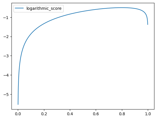
Now it’s time to try this out! The observations that we have generated have resulted in an ideal rain prediction of \(p = 0.80095\). Since we have a step of 0.001 the closest probability that we will test is 0.801.
The plot shows me that the score rule peaks around 0.8 and we can confirm that the very best value is \(p = 0.801\). This has worked out.
Now we can try evaluating some other score functions. To start with we can try removing the logarithm from the function. This is a monotonic transformation as if \(x > y\) then \(\ln (x) > \ln (y)\).
Code
import numpy as npdef linear_score(p: float, x: np.array) ->float: scores = x * p scores += (1- x) * (1- p)return scores.mean()
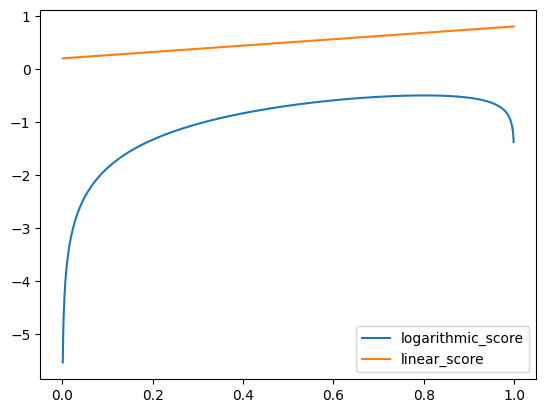
The linear score has clearly failed. What is more interesting is that while the log to linear transformation is monotonic, the mean of that transformation over the observations is not.
We can review the code to find out why - linear_score is now producing the best score at 1 (or 0.999 due to the range of tests). If we substitute this into the function we can see it becomes \(\frac{1}{N} \sum^i_N ( x_i \cdot 1 + (1 - x_i) \cdot 0 )\) which becomes \(\frac{1}{N} \sum x = 0.80095\). When comparing this to the closest tested probability of 0.801 the function becomes \(\frac{1}{100,000} \cdot ( 80095*0.801 + 19905*0.199 ) = 0.6811719\). The problem is the multiplication of \(p\) with \(x\) results in reducing the benefit of being close to the true probability.
This was a nice demonstration that monotonic transformations to a proper scoring rule do not always produce a proper scoring rule.
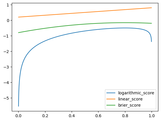
Another scoring rule which wikipedia states is proper is the Brier or quadratic score. We can compare this.
Code
import numpy as npdef brier_score(p: float, x: np.array) ->float: scores = (x - p) **2return-scores.mean() # orientation of brier is inverted
The Brier score is much smoother than the logarithmic score, and as expected the probability with the best score is the one closest to the true value.
Is Brier better than logarithmic? What makes a scoring rule good? There are an infinite number of proper scoring rules. Having some ideals or desires around these rules could help.
Best Scoring Rule
I’ve just started learning about these, so how could I come up with a feel for a good rule?
One thing might be to consider how they behave when you are extremely wrong. What happens if we predict a 100% chance of rain, and subsequently it does not rain? The logarithm of 0 is undefined, but it tends towards infinity.
My collegue linked me this blog post about proper scoring rules and it has a comparison of logarithmic scoring and Brier scoring (calling them log loss and mean square error). In it the writer defines two criteria that a good scoring rule should not have. They are:
the insensitivity property, which is essentially about how once a scorer has been penalized by infinity, it doesn’t matter how well they perform on the rest of their predictions
(the) hypersensitivity (property), which is that the asymptote becomes very extreme very quickly. Selton writes that this “implies the value judgment that small differences between small probabilities should be taken very seriously and that wrongly describing something extremely improbable as having zero probability is an unforgivable sin.”
These two critera are problematic for the logarithmic scoring rule, but not the Brier rule. That would be a reason to choose Brier.
Cross Entropy Loss
Cross Entropy Loss is widely used when training deep learning models. Is cross entropy a proper scoring rule? Is cross entropy more like the logarithmic rule or the Brier rule?
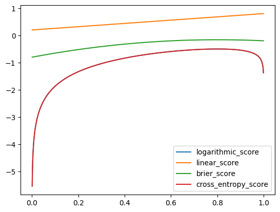
We can start by looking at it on the plot and then breaking down the code. One problem is that cross entropy implicitly involves a softmax. The equation for softmax is \(\frac{e^{x_i}}{\sum_i e^{x_i}}\), given this it should be enough to take the log to reverse the exponent.
Code
import numpy as npimport torchdef cross_entropy_score(p: float, x: np.array) ->float: x_tensor = torch.from_numpy(x) p_tensor = torch.zeros(x.shape[0], 2) p_tensor[:, 0] =1- p p_tensor[:, 1] = p p_tensor = p_tensor.log() # invert softmax loss = torch.nn.functional.cross_entropy(input=p_tensor, target=x_tensor, reduction="mean", )return-loss.item()
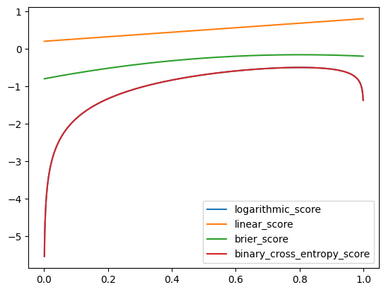
Here we can see that the cross entropy score perfectly overlaps the original logarithmic score on the plot. That’s quite satisfying, however it does mean that cross entropy loss suffers from the precise problems that we just discussed - it can produce an infinite loss, and a small change in probability (e.g. from low probability to zero) can result in a very large change in loss.
Given all of this, why is cross entropy loss used so much? Secondly language models use cross entropy to train. Using cross entropy results in the language models being poorly calibrated and over confident in their predictions. This is the opposite of what I would expect given the criteria from that blog post.
What is the deal with Cross Entropy Loss?
Shouldn’t cross entropy loss produce an infinite value for a completely wrong answer? Can we test this? Is it possible for a single softmax to produce zero for one of the values?
Code
import pandas as pdpd.DataFrame([ {"ratio": value,"big": torch.tensor([value, 1], dtype=float).softmax(-1)[0].item(),"small": torch.tensor([value, 1], dtype=float).softmax(-1)[1].item(), }for value in [1, 1e1, 1e2, 1e3]])
ratio
big
small
0
1.0
0.500000
5.000000e-01
1
10.0
0.999877
1.233946e-04
2
100.0
1.000000
1.011221e-43
3
1000.0
1.000000
0.000000e+00
This is an achievable difference in output value for a model, although a little large. Let’s see what cross entropy loss gives us for such a range.
import torchloss = torch.nn.CrossEntropyLoss()(input=torch.tensor([[1e3, 0]], dtype=float), target=torch.tensor([1], dtype=int),)print(f"The loss for incorrectly predicting [1000, 0] is {loss.item()}")
The loss for incorrectly predicting [1000, 0] is 1000.0
This is the difference between the two values. I wonder what it is like for a larger value.
import torchloss = torch.nn.CrossEntropyLoss()(input=torch.tensor([[1e30, 0]], dtype=float), target=torch.tensor([1], dtype=int),)print(f"The loss for incorrectly predicting [1e30, 0] is {loss.item()}")
The loss for incorrectly predicting [1e30, 0] is 1e+30
It seems like the potential loss from cross entropy isn’t infinite, instead is the difference between the values. In these extreme cases cross entropy loss is not hypersensitive, as the change in loss is linear compared to the difference in prediction.
So why do we see the extreme curve when plotting the score? I think that reversing the softmax has caused the log to become linear (which makes a lot of sense really). Is there another loss function which does not incorporate the softmax?
I use cross entropy loss to train a model when there is a single correct answer. If there are multiple correct answers (or none) then I use binary cross entropy loss. Binary cross entropy does not incorporate softmax, instead requiring that all of the inputs be in the range \([0, 1]\) as each input is the probability of that class being present. Can we try that?
Code
import numpy as npimport torchdef binary_cross_entropy_score(p: float, x: np.array) ->float: x_tensor = torch.zeros(x.shape[0], 2) x_tensor[range(x_tensor.shape[0]), x] =1 p_tensor = torch.zeros(x.shape[0], 2) p_tensor[:, 0] =1- p p_tensor[:, 1] = p loss = torch.nn.functional.binary_cross_entropy(input=p_tensor, target=x_tensor, reduction="mean", )return-loss.item()
The lack of scaling for binary cross entropy means that we should be able to prove that it is hypersensitive. Can we get binary cross entropy loss to produce an extreme output?
Code
import torchloss = torch.nn.functional.binary_cross_entropy(input=torch.tensor([[0.]]), target=torch.tensor([[1.]]), reduction="mean",)print(f"The loss of a 100% incorrect prediction is {loss.item()}")loss = torch.nn.functional.binary_cross_entropy(input=torch.tensor([[0.01]]), target=torch.tensor([[1.]]), reduction="mean",)print(f"The loss of a 99% incorrect prediction is {loss.item()}")loss = torch.nn.functional.binary_cross_entropy(input=torch.tensor([[0.02]]), target=torch.tensor([[1.]]), reduction="mean",)print(f"The loss of a 98% incorrect prediction is {loss.item()}")
The loss of a 100% incorrect prediction is 100.0
The loss of a 99% incorrect prediction is 4.605170249938965
The loss of a 98% incorrect prediction is 3.9120230674743652
This clearly shows that binary cross entropy is hypersensitive, as a 1% change in probability has been shown to be either a ~95 increase in loss or a ~0.7 increase in loss. What is more interesting is that the loss of being exactly wrong is not infinite. 100% wrong is the most incorrect you can be and the loss is “only” 100. Why is this? The documentation for BCELoss explicitly states that:
For one, if either \(y_n=0\) or \((1−y_n)=0\), then we would be multiplying 0 with infinity. Secondly, if we have an infinite loss value, then we would also have an infinite term in our gradient, since \(\lim_{x \to 0} \frac{d}{dx} \log(x) = \infty\). This would make BCELoss’s backward method nonlinear with respect to \(x_n\), and using it for things like linear regression would not be straight-forward.
Our solution is that BCELoss clamps its log function outputs to be greater than or equal to -100. This way, we can always have a finite loss value and a linear backward method.
Forcing the output to be limited prevents the loss from being overwhelmed by a single completely incorrect prediction. I have to wonder if patching the loss function like this is ideal.
A further question that I have is why deep learning models tend to be poorly calibrated (Guo et al. 2017), (Wang 2023). The best loss achievable is provably when the model makes the prediction closest to the true distribution.
Guo, Chuan, Geoff Pleiss, Yu Sun, and Kilian Q. Weinberger. 2017. “On Calibration of Modern Neural Networks.”https://arxiv.org/abs/1706.04599.
I wonder if the over calibration is due to the difference between individual predictions and aggregated predictions - for any individual observation the best loss is to match the outcome exactly instead of matching the distribution. The way that models are trained gives them per-batch updates which would encorage movement towards this individual prediction maximum as the distribution for the specific prediction being made is not present in the batch.
It would be interesting to try to address this. I wonder if the fix would be to create larger batches that show the distribution of a given prediction more directly. It’s likely that such a setup would be far more costly to train, as you wouldn’t want contributions from the other words in each row. Fully training a modern language model is already out of my reach so this is more of a thought experiment right now.