Matthew’s Blog - KL Divergence and Scoring Rules

In the previous post we went over scoring rules and compared the logarithmic scoring rule to the Brier scoring rule. Both of these rules are proper however the logarithmic scoring rule can result in an infinitely bad score for a completely wrong prediction. This lead me to believe that the Brier scoring rule is better.

When training deep learning models I frequently use cross entropy loss or binary cross entropy loss. Comparing these loss functions to the scoring rules I found that they are directly equivalent to the logarithmic scoring rule. Why would these be the most prevalent loss functions when it has the ability to exponentially punish being very wrong? Large language models are trained using cross entropy loss after all.

I discussed this with a friend and he made a strong statement. He said that every time someone uses cross entropy loss they have made a mistake and instead should be using Kullback-Leibler divergence loss (Kullback and Leibler 1951) (commonly referred to as KL div loss). He knows a lot about mathematics and so this assertion interests me.

Kullback, S., and R. A. Leibler. 1951. “On Information and Sufficiency.” The Annals of Mathematical Statistics 22 (1): 79–86. https://doi.org/10.1214/aoms/1177729694.

KL Divergence and Cross Entropy

KL Divergence is defined as:

\[ D_\text{KL}(P \parallel Q) = \sum_{x\in\mathcal{X}} P(x) \log\left(\frac{P(x)}{Q(x)}\right) \]

\(P\) is the actual distribution (i.e. the observed reality) and \(Q\) is the predicted distribution (i.e. the model output).

We can expand this out to become:

\[ \begin{aligned} D_\text{KL}(P\parallel Q) &= \sum_{x\in\mathcal{X}} p(x) \log (p(x)) - \sum_{x\in\mathcal{X}} p(x) \log (q(x)) \\ &= (-\text{H}(P)) - (-\text{H}(P, Q)) \end{aligned} \]

(On wikipedia the expansion is expressed as \(\log\left(\frac{1}{p(x)}\right)\) to avoid all the negation in the equivalence.)

This formulation is relevant because the \(\text{H}(P, Q)\) term is cross entropy:

\[ H(P,Q) = -\sum_{x\in\mathcal{X}} p(x)\, \log (q(x)) \]

This means that the difference between KL Divergence and cross entropy is the inclusion of the \(\text{H}(P)\) term, which is the entropy of the actual distribution.

As a side note it’s fun to write the math out as it then shows that the logarithmic scoring rule is cross entropy negated.

What effect does including the entropy of the actual distribution have? How does this handle extremely incorrect predictions? Let’s find out.

Empirical Comparison

We can use the code from the previous post to compare KL divergence to cross entropy and logarithmic score. In the previous post we could use this to show that cross entropy and logarithmic score was equivalent. The same set of observations will be used so we can compare this directly to the previous version.

Code

from scipy.stats import bernoulli
import numpy as np
import pandas as pd
from textwrap import wrap

rain_probability = 0.8
observations = bernoulli.rvs(
    rain_probability,
    size=100_000,
    random_state=42,
)

print(
    "\n".join(
        wrap(
            f"generated {len(observations):,} weather observations "
            f"with a probability of rain of {observations.mean()}",
            width=40,
        )
    )
)

def logarithmic_score(p: float, x: np.array) -> float:
    scores = x * np.log(p)
    scores += (1 - x) * np.log(1 - p)
    return scores.mean()

def evaluate_score(score_function, x: np.array, step: float = 0.001) -> pd.Series:
    probabilities = np.arange(step, 1, step)
    values = pd.Series([
        score_function(p=p, x=x)
        for p in probabilities
    ], index=probabilities)
    return values.to_frame("score")

def evaluate_scores(functions: list, x: np.array, step: float = 0.001) -> pd.DataFrame:
    probabilities = np.arange(step, 1, step)
    scores = {
        score_function.__name__: pd.Series([
            score_function(p=p, x=x)
            for p in probabilities
        ], index=probabilities)
        for score_function in functions
    }
    return pd.DataFrame(scores)

def show_best(df: pd.DataFrame) -> pd.DataFrame:
    best_rows = {
        column: df.iloc[df[column].argmax()]
        for column in df.columns
    }
    return pd.DataFrame([
        {
            "name": column,
            "probability": row.name,
            "score": row[column],
        }
        for column, row in best_rows.items()
    ])

generated 100,000 weather observations
with a probability of rain of 0.80095

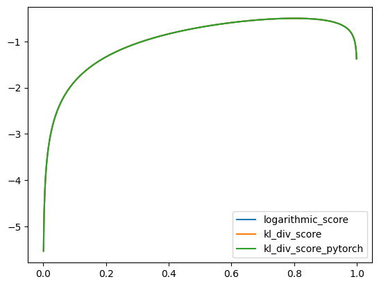
Now I can write two implementations of KL Divergence. The first will use scipy.special.xlogy and the second will use the pytorch kl_div function.

To do this correctly the KL divergence has to be run over the rain outcome and the dry outcome. This is equivalent to the two terms in the logarithmic score rule: \(\underbrace{x \log(x)}_\text{rain} + \underbrace{(1 - x) \log(1 - x)}_{\text{dry}}\).

Code

from scipy.special import xlogy
import numpy as np
import torch

def kl_div_score(p: float, x: np.array) -> float:
    kl_div = lambda p, x: xlogy(x, x) - xlogy(x, p)
    scores = kl_div(p, x) + kl_div(1 - p, 1 - x)
    return -scores.mean()

def kl_div_score_pytorch(p: float, x: np.array) -> float:
    x_tensor = torch.from_numpy(x)[:, None].float()
    x_tensor = torch.concat([x_tensor, 1. - x_tensor], dim=1)
    p_tensor = torch.full((len(x), 1), p)
    p_tensor = torch.concat([p_tensor, 1 - p_tensor], dim=1)
    p_tensor = p_tensor.log()
    loss = torch.nn.functional.kl_div(
        input=p_tensor,
        target=x_tensor,
        reduction="batchmean",
    )
    return -loss.item()

values = evaluate_scores(
    [
        logarithmic_score,
        kl_div_score,
        kl_div_score_pytorch,
    ],
    x=observations,
    step=0.001,
)

values.plot()
show_best(values)

	name	probability	score
0	logarithmic_score	0.801	-0.499083
1	kl_div_score	0.801	-0.499083
2	kl_div_score_pytorch	0.801	-0.499083

In this graph we have three plots but only one line. That’s because they all perfectly match each other. We can see that the two implementations of KL divergence match the logarithmic score.

Mathematical Comparison

Can we prove that cross entropy and kl divergence are equivalent? To do this we would have to demonstrate that the new term in KL divergence is always zero. That is the only way it could have no effect as it is added to the Cross Entropy value.

In our example we have two observations, rain and dry. We represent these with \(1\) for rain and \(0\) for dry.

The additional term is \(H(\mathcal{X}) = - \sum_{x\in\mathcal{X}} p(x) \log (p(x))\). For an individual observation we can substitute in the two values to see how they work out:

\[ \begin{aligned} H(x) &= p(x) \log p(x) \\ H(rain) &= p(x_{rain}) \log (p(x_{rain})) &= 1 \log (1) &= 1 \cdot 0 \\ H(dry) &= p(x_{dry}) \log (p(x_{dry})) &= 0 \log (0) \end{aligned} \]

With the observation that \(\lim_{x \to 0^{+}} x \log(x) = 0\) we can see that both the \(H(rain)\) and \(H(dry)\) observations result in an additional term of zero.

When would KL divergence diverge from Cross Entropy loss? I think it would require a continuous observed distribution. This means that there are plenty of training situations where KL divergence adds nothing.

Comparison by Others

My colleague also found this stats stackoverflow question which asks what the difference is. There are a variety of different answers to this which can be summarized as:

#1 If the additional term that KL divergence provides is a constant then minimizing KL divergence is equivalent to minimizing Cross Entropy. This is what we have just explored.

There is an interesting comment which notes that the goal of machine learning models is to make predicted distribution as close as possible to the fixed [true distribution]. This makes me question the value of the additional term - if we want to match the true distribution, no matter how complex, then what is the benefit of measuring the distribution?
#2 and #4 For training deep learning models the additional parameter is measured over the minibatch. This makes it less stable.

There is even a comment mentioning that KL divergence was less robust than Binary Cross Entropy when training a model. The contrasting answer states that the gradient of the additional term is zero as it is not based on the output of the model. It would be very interesting to test this.

Can KL Divergence alter Back Propagation?

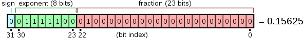
Training deep learning models can be described mathematically, which we have done above. It also intimately involves the implementation in software. Numbers are represented using IEEE 754 floating point representation which splits the number into a significand and an exponent:

\[ N = N_{significand} \cdot N_{base}^{N_{exponent}} \]

The example in wikipedia is:

\[ \begin{aligned} 12.345 &= 12345 \cdot 10^{-3} \\ N_{significand} &= 12345 \\ N_{base} &= 10 \\ N_{exponent} &= -3 \end{aligned} \]

The base is defined by the IEEE 754 standard and is either 2 or 10. The base is set by the number format and is not represented in the bits of the float itself. You can see how a 32 bit float is encoded with this image from wikipedia:

All of this matters because representing any real number in a fixed format inevitably involves a loss of precision. The floating point format has this problem when the difference between the exponent of two numbers is too large. If those numbers are added then the value with the smaller exponent will have no resulting effect on the final value.

We can determine the smallest value that we can add to a number and produce a change. I’ve heard this called the ulp which is the smallest difference between a given floating point value and any other distinct floating point value. It is called the unit in last place because it is the change in quantity represented by flipping the last (zeroeth) bit in the float.

In python there is the math.ulp which calculates this. It’s easy to calculate this manually, so we can see how it works:

import math
from textwrap import wrap

def my_ulp(value: float) -> float:
    difference = value
    while value + difference != value:
        difference = difference / 2
    return difference * 2

if math.ulp(1.0) == my_ulp(1.0):
    print("The math.ulp code is equivalent to my_ulp for the value 1.0\n")

one_after = 1.0 + math.ulp(1.0)
still_one_after = 1.0 + (math.ulp(1.0) * 0.9)

if one_after == still_one_after:
    print("\n".join(wrap(
        "The math.ulp value is the smallest representable difference. "
        "You can still add a smaller number and produce a difference "
        "due to rounding"
    )), "\n")

half_after = 1.0 + math.ulp(1.0) / 2
if 1.0 == half_after:
    print("Half of the math.ulp is small enough to make no difference\n")

one_ulp = math.ulp(1.0)
one_billion_ulp = math.ulp(1e9)

if one_ulp < one_billion_ulp:
    print("The math.ulp value gets bigger as the number grows\n")

The math.ulp code is equivalent to my_ulp for the value 1.0

The math.ulp value is the smallest representable difference. You can
still add a smaller number and produce a difference due to rounding 

Half of the math.ulp is small enough to make no difference

The math.ulp value gets bigger as the number grows

The significance of this is that we can produce a difference between the two terms of the KL divergence loss that is so big that the Cross Entropy term contributes nothing to the final value. Then we can test if the gradient produced by that differs from the gradient produced by Cross Entropy.

As we have established a value that is smaller than half of the ulp value will be small enough. What prediction and observation can produce a large enough difference? Since we are interested in implementation details I am not concerned about restricting this to true probability distributions.

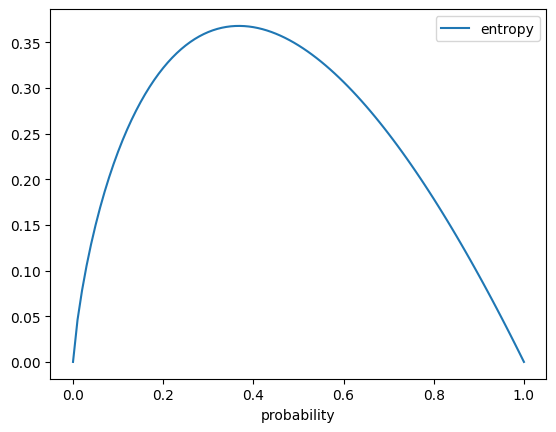
The first thing to do is to maximize the \(H(P)\) term. We can graph it and then calculate the maximum value.

Code

import pandas as pd
from scipy.special import xlogy
import numpy as np

df = pd.DataFrame([
    {
        "probability": probability,
        "entropy": -xlogy(probability, probability),
    }
    for probability in np.arange(0, 1.01, 0.01)
])
df = df.set_index("probability")

df.plot()
df.iloc[df.entropy.argmax()].to_frame()

	0.37
entropy	0.367873

The equation we are working with is \(x log(x)\) and we can calculate the maximum entropy by taking the derivative of it. I don’t do derivatives often so I’m going to write this all out.

\[ \frac{d}{dx} \left( x \log(x) \right) \]

We have two terms that are multiplied, so we use the product rule \(( f \cdot g )' = f' \cdot g + f \cdot g'\). This means we need to calculate the derivative of the two terms:

\[ \begin{aligned} \frac{dx}{dx} &= 1 \\ \frac{d}{dx} \left( \log(x) \right) &= \frac{1}{x} \end{aligned} \]

The derivative is then:

\[ \begin{aligned} \frac{dx}{dx} \cdot \log(x) + x \cdot \frac{d}{dx} \left( \log(x) \right) &= 1 \cdot \log(x) + x \cdot \frac{1}{x} \\ &= \log(x) + 1 \end{aligned} \]

To find the maximum point of the original equation we solve this for zero:

\[ \begin{aligned} \log(x) + 1 &= 0 \\ \log(x) &= -1 \\ x &= e^{-1} \\ x &= \frac{1}{e} \end{aligned} \]

We can now make a distribution with the largest possible entropy by using \(\frac{1}{e}\) as our expected probability. I should do this more often.

The next question is how can we minimize the cross entropy of \(x \log (y)\). It’s easy this time as we can use a \(y\) of 1, as \(\log(1) = 0\).

That then produces the following:

import math
from scipy.special import xlogy

distribution = 1 / math.e
prediction = 1.

distribution_entropy = xlogy(distribution, distribution)
cross_entropy = xlogy(distribution, prediction)

print(f"prediction:           {prediction}")
print(f"distribution entropy: {distribution_entropy:g}")
print(f"cross entropy:        {cross_entropy:g}")

prediction:           1.0
distribution entropy: -0.367879
cross entropy:        0

A contribution of 0 for the cross entropy isn’t helpful though as we do want an infintesimal value to establish that there is a difference between the theoretical and practical outcomes.

Code

import math
from scipy.special import xlogy

distribution = 1 / math.e
prediction = 1. - math.ulp(1.)

distribution_entropy = xlogy(distribution, distribution)
cross_entropy = xlogy(distribution, prediction)

print(f"prediction:           {prediction}")
print(f"distribution entropy: {distribution_entropy:g}")
print(f"cross entropy:        {cross_entropy:g}")

if cross_entropy != 0:
    print("cross entropy is distinct from zero")
if distribution_entropy + cross_entropy == distribution_entropy:
    print("adding cross entropy results in no change to the overall entropy value")
else:
    print("adding cross entropy results in a change to the overall entropy value")

prediction:           0.9999999999999998
distribution entropy: -0.367879
cross entropy:        -8.16856e-17
cross entropy is distinct from zero
adding cross entropy results in a change to the overall entropy value

We have a problem here. The cross entropy value exceeds the minimal change threshold for the overall entropy value.

We can still achieve our goal by getting further into the specific implementation that pytorch uses for KL div. Our problem is that the logarithm of the minimally different value is no longer minimally different from zero. The pytorch implementation of KL div expects the prediction to be in log space. With this I can then force the prediction to be arbitrarily close to zero.

With this knowledge we can test our different example predictions. To see what the gradient will be we can train the prediction directly by making it a parameter and using an optimizer. This will cause the prediction to get updated and the gradient on that prediction will be set.

To start with we can work with a sensible prediction to check this all works:

Code

import math
import torch
from torch.nn import functional as F

distribution = torch.tensor([[1 / math.e]])
prediction = torch.nn.Parameter(
    torch.tensor([[0.5]])
)
optim = torch.optim.SGD([prediction], lr=0.1)

optim.zero_grad()
loss = -F.kl_div(
    input=prediction.log(),
    target=distribution,
    reduction="batchmean",
)
loss.backward()
optim.step()

print(f"prediction is:     0.5")
print(f"loss is:           {loss.item():g}")
print(f"gradient is:       {prediction.grad.item():g}")
print(f"new prediction is: {prediction.data.item():g}")

prediction is:     0.5
loss is:           0.112885
gradient is:       0.735759
new prediction is: 0.426424

Now we can try an extreme prediction, remembering that the prediction is now in log space:

Code

import math
import torch
from torch.nn import functional as F

distribution = torch.tensor([[1 / math.e]])
# prediction is now log space
prediction = torch.nn.Parameter(
    torch.tensor([[1e-30]])
)
optim = torch.optim.SGD([prediction], lr=0.1)

optim.zero_grad()
loss = -F.kl_div(
    input=prediction,
    target=distribution,
    reduction="batchmean",
)
loss.backward()
optim.step()

print(f"log prediction is: 1e-30")
print(f"loss is:           {loss.item():g}")
print(f"gradient is:       {prediction.grad.item():g}")
print(f"new prediction is: {prediction.data.item():g}")

log prediction is: 1e-30
loss is:           0.367879
gradient is:       0.367879
new prediction is: -0.0367879

We can see that the gradient is still present, even though the loss value is unaffected by the Cross Entropy term (separately it’s quite odd that it has moved the prediction in the wrong direction).

We can check the gradient is only related to the Cross Entropy term by testing \(y \log(x)\) over the same values:

Code

import math
import torch
from torch.nn import functional as F

distribution = torch.tensor([[1 / math.e]])
# prediction is now log space
prediction = torch.nn.Parameter(
    torch.tensor([[1e-30]])
)
optim = torch.optim.SGD([prediction], lr=0.1)

optim.zero_grad()
loss = distribution * prediction
loss.backward()
optim.step()

print(f"log prediction is: 1e-30")
print(f"loss is:           {loss.item():g}")
print(f"gradient is:       {prediction.grad.item():g}")
print(f"new prediction is: {prediction.data.item():g}")

log prediction is: 1e-30
loss is:           3.67879e-31
gradient is:       0.367879
new prediction is: -0.0367879

The resulting gradient and change to the prediction is identical. We can also see now that the loss of the cross entropy is small enough to make no change to the overall loss. This establishes that the gradient calculations in pytorch are independent of the actual loss value involved.

With all this the question remains - should KL divergence be used over Cross Entropy? Broadly there is a problem here, as only the Cross Entropy term involves the output of the model and so that is the only part that will actually affect the model through back propagation.

Predicting Never

A prediction of 0 means never. A prediction of 1 means always.

These are extreme predictions. My friend suggested to me that any model which makes such an extreme prediction is not really making a prediction, instead it is expressing a constraint. If the model expresses such a constraint, and the constraint does not hold, then the model is fundamentally unsuitable.

This is not a new idea, and my work colleague mentioned Cromwell’s rule in regard to this:

Cromwell’s rule … states that the use of prior probabilities of 1 (“the event will definitely occur”) or 0 (“the event will definitely not occur”) should be avoided, except when applied to statements that are logically true or false, such as 2+2 equaling 4.

The reference is to Oliver Cromwell, who wrote to the General Assembly of the Church of Scotland on 3 August 1650, shortly before the Battle of Dunbar, including a phrase that has become well known and frequently quoted:

I beseech you, in the bowels of Christ, think it possible that you may be mistaken.

As Lindley puts it, assigning a probability should “leave a little probability for the moon being made of green cheese; it can be as small as 1 in a million, but have it there since otherwise an army of astronauts returning with samples of the said cheese will leave you unmoved.”

This would permit an infinite punishment for a completely wrong prediction. However we have just covered a situation where the practical constraints of deep learning systems make some measurements indistinguishable from zero. If we do have a model that is actively being trained then producing the completely wrong answer is a learning opportunity instead of an unforgivable error. For this reason I can support limiting the maximum loss.

If we recall the two value judgements for scoring rules:

the insensitivity property, which is essentially about how once a scorer has been penalized by infinity, it doesn’t matter how well they perform on the rest of their predictions

(the) hypersensitivity (property), which is that the asymptote becomes very extreme very quickly. Selton writes that this “implies the value judgment that small differences between small probabilities should be taken very seriously and that wrongly describing something extremely improbable as having zero probability is an unforgivable sin.”

Clipping the maximum loss addresses the insensitivity problem. The exponential curve of the scores as they approach a completely wrong prediction are still hypersensitive. Nothing that I have covered in this post really addresses that or compares using a loss function like mean squared error which is not hypersensitive. It would be interesting to try that out.