How is Cosine Similarity affected by dimension count

A paper recently used a cosine similarity of 0.5 to cluster news articles. This seemed like a high value to me as cosine similarity itself has a range of -1 to 1. The vectors that were being clustered were \(x \in \mathbb{R}^{768}\), so they were of reasonably high dimensionality.

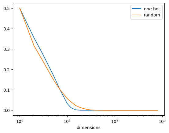
How does the number of matches with this threshold vary as we increase the dimension count? We can test this in two ways, one with a fixed one hot vector compared to a random vector, and another with two random vectors.

Code

import numpy as np
from sklearn.metrics.pairwise import cosine_similarity

def compare_one_hot(dimensions: int, iterations: int, threshold: float = 0.5) -> float:
    target = np.zeros((1, dimensions))
    target[:, 0] = 1.
    comparison = np.random.uniform(low=-1., high=1., size=(iterations, dimensions))
    distance = cosine_similarity(comparison, target)
    matching = distance >= threshold
    return matching.sum() / iterations

def compare_random(dimensions: int, iterations: int, threshold: float = 0.5) -> float:
    target = np.random.uniform(low=-1., high=1., size=(1, dimensions))
    target[:, 0] = 1.
    comparison = np.random.uniform(low=-1., high=1., size=(iterations, dimensions))
    distance = cosine_similarity(comparison, target)
    matching = distance >= threshold
    return matching.sum() / iterations

Code

import pandas as pd

dimensions = sorted({
    int(10**log_d)
    for log_d in np.arange(0, 3, 0.1)
})
df = pd.DataFrame([
    {
        "dimensions": n,
        "one hot": compare_one_hot(
            dimensions=n,
            iterations=100_000,
            threshold=0.5,
        ),
        "random": compare_random(
            dimensions=n,
            iterations=100_000,
            threshold=0.5,
        ),
    }
    for n in dimensions
])
df = df.set_index("dimensions")

df.plot(logx=True)
df.iloc[[0, -1]]

	one hot	random
dimensions
1	0.50081	0.50064
794	0.00000	0.00000

We can see that as the dimension count increases the probability decreases. By the time you reach the high dimensions there are very few matches (0 matches in 100,000 comparisons). So it is a discriminatory test. Why is this?

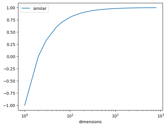
If we imagine a pair of vectors and the similarity between them, can we produce a positive cosine similarity if any of the dimensions are orthogonal? Cosine similarity is the normalized dot product of the two vectors. The most similar vector pair with orthogonality would be \([1, ...]^N\) and \([-1, 1, ...]^N\). Let’s compare these.

Code

import numpy as np
from sklearn.metrics.pairwise import cosine_similarity

def compare_similar(dimensions: int) -> float:
    all_ones = np.ones((1, dimensions))
    all_but_one = np.ones((1, dimensions))
    all_but_one[0, 0] = -1
    distance = cosine_similarity(all_ones, all_but_one)
    return distance[0, 0]

Code

import pandas as pd

dimensions = sorted({
    int(10**log_d)
    for log_d in np.arange(0, 3, 0.1)
})
df = pd.DataFrame([
    {
        "dimensions": n,
        "similar": compare_similar(dimensions=n),
    }
    for n in dimensions
])
df = df.set_index("dimensions")

df.plot(logx=True)
df.iloc[[0, -1]]

	similar
dimensions
1	-1.000000
794	0.997481

Here we can see that the dimensionality works in our favour. Why then does the random comparison end up punishing us so much?

Can we work out what the threshold is for the matching pairs such that we get at least 0.5 similarity?

Code

import numpy as np
from sklearn.metrics.pairwise import cosine_similarity

def required_matches(dimensions: int, threshold: float = 0.5) -> float:
    target = np.ones((1, dimensions))
    comparison = np.zeros((1, dimensions))
    comparison[0, 0] = -1
    for n in range(0, dimensions):
        if n != 0:
            comparison[0, n] = 1
        distance = cosine_similarity(target, comparison)[0,0]
        if distance >= threshold:
            return n
    return np.inf

Code

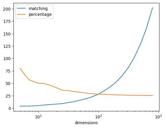
import pandas as pd

dimensions = sorted({
    int(10**log_d)
    for log_d in np.arange(0, 3, 0.1)
})
df = pd.DataFrame([
    {
        "dimensions": n,
        "matching": required_matches(dimensions=n),
        "percentage": required_matches(dimensions=n) * 100 / n,
    }
    for n in dimensions
])
df = df.set_index("dimensions")

df.plot(logx=True)
df.iloc[[0, 1, 2, 3, -1]]

	matching	percentage
dimensions
1	inf	inf
2	inf	inf
3	inf	inf
5	4.0	80.000000
794	202.0	25.440806

What this graph is showing me is that a single orthogonal value becomes increasingly impactful as the number of dimensions increases. In order to counteract a single orthogonal value a large percentage of the remaining values must match. This becomes increasingly unlikely as the number of dimensions grows.

Expressing this relationship mathematically might be interesting. For now I’m going to get on with other things.