Detecting NPCs in Old School Runescape

Detecting NPCs

Old school runescape is an old mmo which relies on grinding statistics for hours on end. Once you’ve done that you can engage in some parts of the game that would otherwise be impossible. A lot of mmos rely on this to keep people playing, possibly dressing it up slightly to make it less obvious.

My friend has been playing old school runescape (osrs) for years now and wanted to apply some programming to make the grind easier. I don’t really have a problem with this, for me he is just changing the game.

The client for osrs is called runelite and is written in Java. There are many plugins for it which can link directly to the underlying game code. This means that you can draw direct loops around NPCs:

npcs with loops

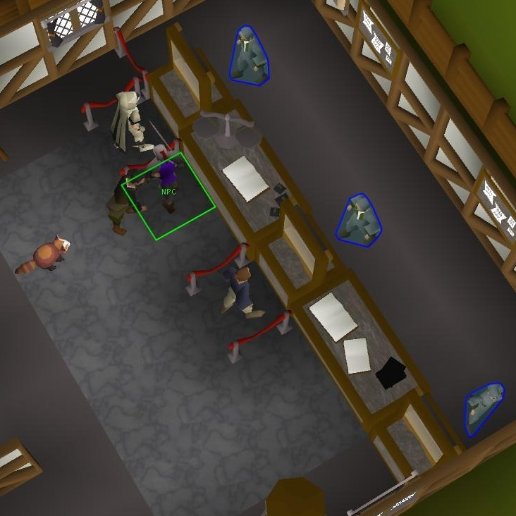
Can we detect the NPCs by detecting these loops?

Convolutions

I like deep learning so I’m going to use convolutions to detect the loops. This is a bit of overkill as you’ll find out.

A convolution takes a part of the image and multiplies it by a set of numbers. These are then summed to produce the output.

To try to visualize this we might think of the pointwise matrix multiplication:

\[ \left[ \begin{matrix} Input_{(0,0)} & ... & Input_{(n,0)} \\ ... & ... & ... \\ Input_{(0,m)} & ... & Input_{(n,m)} \end{matrix} \right] * \left[\begin{matrix} Weight_{(0,0)} & ... & Weight_{(n,0)} \\ ... & ... & ... \\ Weight_{(0,m)} & ... & Weight_{(n,m)} \end{matrix} \right] = \left[\begin{matrix} IW_{(0,0)} & ... & IW_{(n,0)} \\ ... & ... & ... \\ IW_{(0,m)} & ... & IW_{(n,m)} \end{matrix} \right] \]

I find it easier if it’s expressed as the sum of sums:

\[ output = \sum_{i \in 0 .. n} \sum_{j \in 0 .. m} Input_{(i, j)} * Weight_{(i, j)} \]

And that’s because the sum of sums correlates more closely to the code:

input = ...
weight = ...

iw = [
    [input[x + x_offset][y + y_offset] * weight[x][y] for y in range(len(weight[x]))]
    for x in range(len(weight))
]
output = sum(iw)

To run this over the whole input we just slide the input window over, by incrementing the x_offset and y_offset used in the input[x + x_offset][y + y_offset] bit.

We can see from this that while the convolution might be small (for example a 3x3 matrix) it has to be applied over the whole image. This means that it can be quite computationally expensive.

As always it’s easier to see this in action. We are going to take the image from above and run some simple convolutions over it.

Code

from PIL import Image

image = Image.open("bankers.jpeg")
image

We need to deal with tensors, so we must be able to convert the image to a tensor. The image is in RGBA format so we expect a 4 x height x width tensor out of this.

Code

from PIL import Image
import torch
from torchvision.transforms.functional import pil_to_tensor

def to_tensor(image: Image.Image) -> torch.Tensor:
    """
    Convert image to tensor.
    The returned shape is channel x height x width.
    The channels are RGBA.
    The RGB channels range from -1 to 1.
    The alpha channel ranges from 0 to 1.
    """
    image = image.convert("RGBA")
    tensor = pil_to_tensor(image)
    tensor = tensor / 255
    tensor[:3] = tensor[:3] * 2
    tensor[:3] = tensor[:3] - 1
    return tensor

def to_image(tensor: torch.Tensor) -> Image.Image:
    """
    Convert tensor to image.
    Tensor is expected to be height x width.
    The tensor values will be scaled such that the minimum is zero and the maximum is 255.
    """
    assert len(tensor.shape) == 2

    tensor = tensor.float()
    tensor = tensor - tensor.min()
    tensor = tensor / tensor.max()
    tensor = tensor * 255
    tensor = tensor.int()

    array = tensor.cpu().numpy()
    array = array.astype("uint8")

    return Image.fromarray(array, "L")

The code to apply the convolution is below.

Code

from PIL import Image
import torch
from torch import nn

@torch.inference_mode()
def to_convolution_1d(tensor: torch.Tensor) -> nn.Conv2d:
    _, columns, rows = tensor.shape

    conv = nn.Conv2d(
        in_channels=1,
        out_channels=1,
        kernel_size=(columns, rows),
        bias=False,
    )
    conv.weight.data[0] = tensor

    return conv

@torch.inference_mode()
def demo_conv_1d(screenshot: torch.Tensor, target: torch.Tensor) -> torch.Tensor:
    target_conv = to_convolution_1d(target)

    target_conv = target_conv.cuda()
    screenshot = screenshot.cuda()

    detections = target_conv(screenshot)
    detections = detections - detections.min()
    detections = detections / detections.max()

    return detections

Now we can come up with two example convolutions. These detect edges, horizontal or vertical. An edge in an image is a sudden change in color intensity so if we just subtract one pixel value from the next horizontally or vertically then we can see when they rapidly change.

Code

horizontal_edges = torch.tensor([
    [ 1],
    [-1],
])
vertical_edges = torch.tensor([
    [ 1,  -1],
])
image_tensor = to_tensor(image)

def apply_1d_conv(convolution: torch.Tensor) -> None:
    output = demo_conv_1d(
        image_tensor[:3].mean(dim=0)[None],
        convolution[None],
    )
    display(to_image(output[0]))

print("horizontal edges convolution")
apply_1d_conv(horizontal_edges)

print("vertical edges convolution")
apply_1d_conv(vertical_edges)

horizontal edges convolution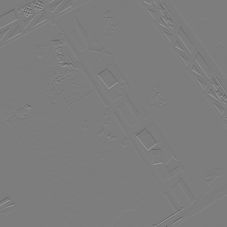

vertical edges convolution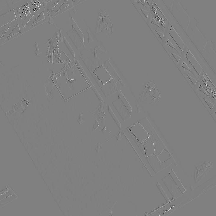

A lot of the edges in this image are diagonal so the two images are quite similar. It is possible to detect edges in any direction using what is called a canny edge detector. You might have fun playing with that.

This is working over the mean of the three RGB channels. We want to detect specific colors though, so can we work over all of the channels? Yes. In the explanation above the additional channel is just another for loop - we do more multiplication and we do more summing.

Code

from PIL import Image
import torch
from torch import nn

@torch.inference_mode()
def to_convolution_demo(tensor: torch.Tensor) -> nn.Conv2d:
    channels, columns, rows = tensor.shape

    conv = nn.Conv2d(
        in_channels=channels,
        out_channels=1,
        kernel_size=(columns, rows),
        bias=False,
    )
    conv.weight.data[0] = tensor

    return conv

@torch.inference_mode()
def demo_conv(screenshot: torch.Tensor, target: torch.Tensor) -> torch.Tensor:
    target_conv = to_convolution_demo(target)

    target_conv = target_conv.cuda()
    screenshot = screenshot.cuda()

    detections = target_conv(screenshot)
    detections = detections - detections.min()
    detections = detections / detections.max()

    return detections

In the following convolutions we just want to detect the primary colors. This has now moved to considering the value of the individual pixels. Given that you could implement this by just operating over the channels directly, which I will demonstrate after.

Code

red_convolution = torch.tensor([
    [[2.]],
    [[-1.]],
    [[-1.]],
])
green_convolution = torch.tensor([
    [[-1.]],
    [[2.]],
    [[-1]],
])
blue_convolution = torch.tensor([
    [[-1.]],
    [[-1]],
    [[2]],
])
blue_convolution = blue_convolution / blue_convolution.std()
image_tensor = to_tensor(image)

def apply_demo_conv(convolution: torch.Tensor) -> None:
    # for deep learning it's very nice to have convolutions with a mean of zero and a standard deviation of 1
    # THIS DOES RESULT IN REDUCING THINGS - a convolution of [0, 0, 3] becomes [-0.5774, -0.5774,  1.1547]
    # you can turn this off if you want to play around with these and explore
    normalized_convolution = convolution - convolution.mean()
    normalized_convolution = normalized_convolution / normalized_convolution.std()

    output = demo_conv(
        image_tensor[:3],
        normalized_convolution,
    )
    display(to_image(output[0]))

print("red 3x1x1 convolution")
apply_demo_conv(red_convolution)
print("green 3x1x1 convolution")
apply_demo_conv(green_convolution)
print("blue 3x1x1 convolution")
apply_demo_conv(blue_convolution)

red 3x1x1 convolution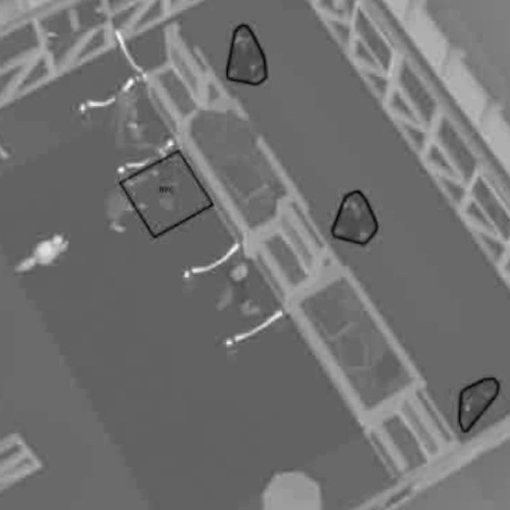

green 3x1x1 convolution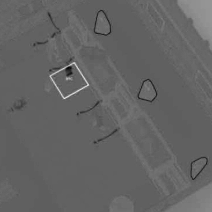

blue 3x1x1 convolution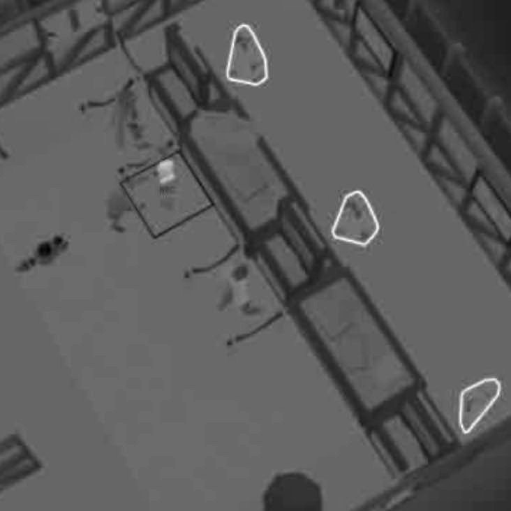

To compare the blue convolution to just summing the different channels:

Code

image_tensor = to_tensor(image)
output = (
    image_tensor[0] * -1.
    + image_tensor[1] * -1.
    + image_tensor[2] * 2.
)
to_image(output)

Summing the different channels produces an image which is functionally identical. This means that you could do everything in numpy if you wanted to. Convolutions are really useful for detecting more significant image features than specific colors.

Anyway, here we can see here that the two runelite additions - the tile border and the NPC borders show up very strongly. The actual game world is quite a mix of colors and is less strongly matched.

This is enough on convolutions now. Let’s see if we can put a bounding box around each of the highlighted NPCs.

Detecting the lasoo

We can see that the blue convolution strongly matches the lasoo around the NPCs. It also matches a few incidental parts of the image.

We want to find the NPCs. How can we do that?

Let’s start by applying the blue convolution and thresholding the output.

Code

import torch

def apply_and_threshold(convolution: torch.Tensor, threshold: float) -> torch.Tensor:
    # for deep learning it's very nice to have convolutions with a mean of zero and a standard deviation of 1
    # THIS DOES RESULT IN REDUCING THINGS - a convolution of [0, 0, 3] becomes [-0.5774, -0.5774,  1.1547]
    # you can turn this off if you want to play around with these and explore
    normalized_convolution = convolution - convolution.mean()
    normalized_convolution = normalized_convolution / normalized_convolution.std()

    output = demo_conv(
        image_tensor[:3],
        normalized_convolution,
    )
    output = output >= threshold
    return output

blue_conv = torch.tensor([
    [[-1.]],
    [[-1]],
    [[2]],
])
image_tensor = to_tensor(image)

# a higher threshold actually perfectly detects the NPCs,
# using a lower one to show the problem.
# denoising is valuable as you are unlikely to have such a clean image to work with in practice.
output = apply_and_threshold(blue_conv, threshold=0.6)
display(to_image(output[0]))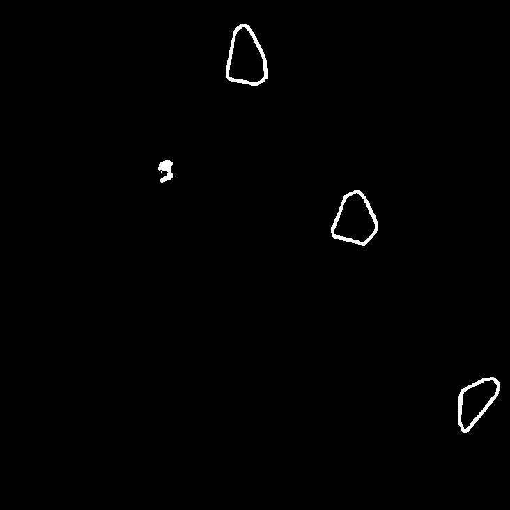

We can see here that the lasoo is strongly matched and that there is some noise (I deliberately lowered the threshold to have something to work with). Removing the noise can be done because the banker lasoo are the biggest continuous clusters of connected pixels. How can we create and filter these clusters?

While you could get clever with algorithms to detect this, I am just going to use an existing clustering algorithm. If we move from the image to trying to cluster the different pixel positions then we should be able to find them quickly. To find the right algorithm we can consider the algorithms available in Scikit learn:

sklearn clustering algorithms and results

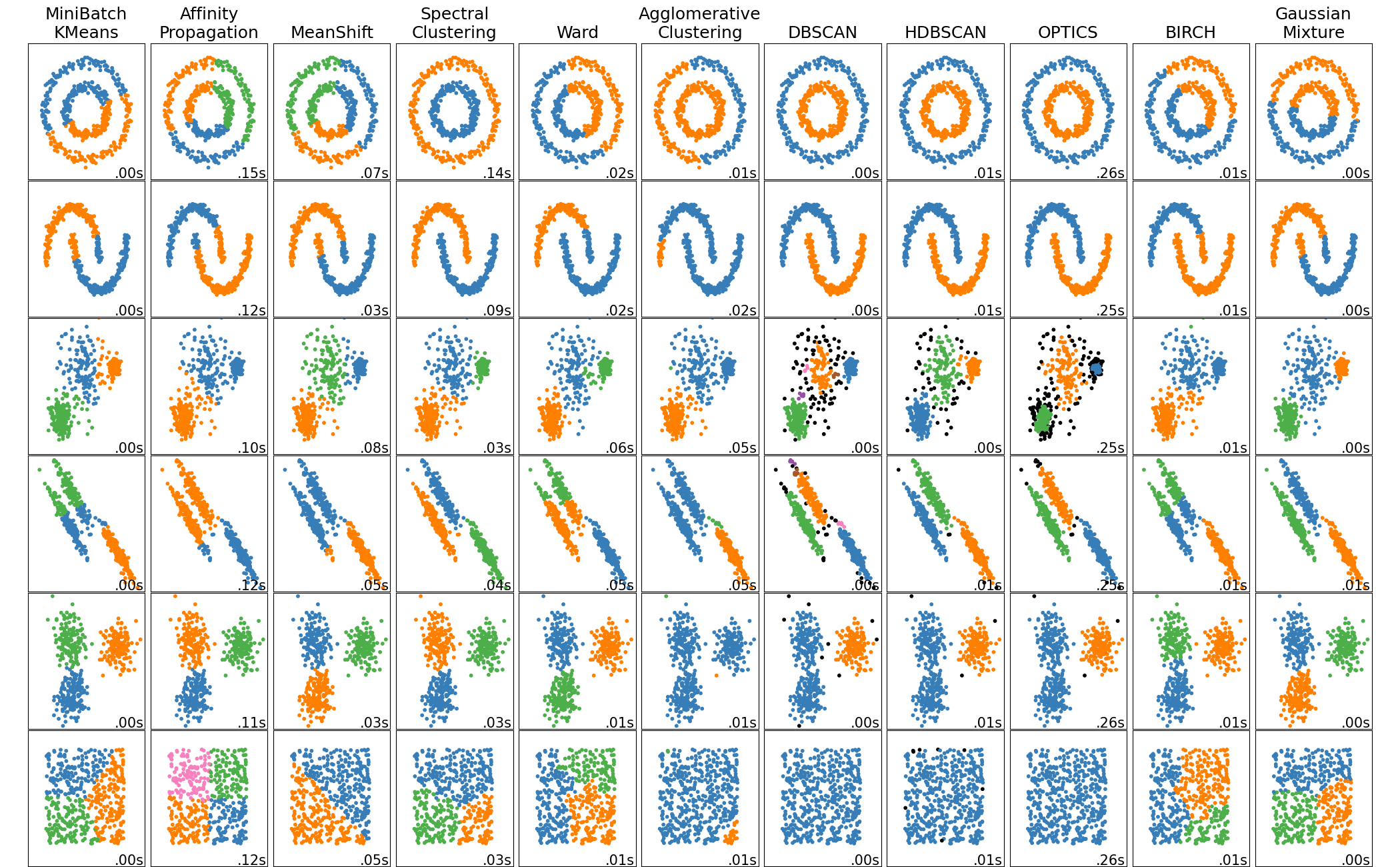
From looking at these it appears that DBSCAN would be good as it detects the continuous lines instead of forming regions out of the space. It’s also one of the fastest, measured at 0.00s.

SciKit Learn DBSCAN

With the nonzero pixels from the image we can use DBSCAN. You can find the documentation here

Since this is a simple operation let’s try using just numpy to spot the loops and scikit learn to cluster them:

Code

from typing import Union
import numpy as np
from PIL import Image

def show_clusters_and_borders(image: np.array, clusters: list[np.array]) -> None:
    print(f"showing {len(clusters)} clusters")

    width, height, _ = image.shape
    filtered_output = np.zeros((width, height), dtype=float)
    for cluster in clusters:
        filtered_output[cluster[:, 0], cluster[:, 1]] = 1
    
        xs = cluster[:, 0]
        ys = cluster[:, 1]
        x_min = xs.min()
        x_max = xs.max()
        y_min = ys.min()
        y_max = ys.max()
    
        filtered_output[x_min:x_max+1, y_min] = 0.5
        filtered_output[x_min:x_max+1, y_max] = 0.5
        filtered_output[x_min, y_min:y_max+1] = 0.5
        filtered_output[x_max, y_min:y_max+1] = 0.5

    display(to_image(torch.from_numpy(filtered_output)))

Code

%%time

from sklearn.cluster import DBSCAN
import numpy as np
from PIL import Image

image = Image.open("bankers.jpeg")

# this image loads as height x width x channel when converted to numpy
image = np.array(image)

# normalize the image to have values between -1 and 1
image = image - image.mean()
image = image / image.max()
image = image * 2
image = image - 1

output = (
    image[:, :, 0] * -1.
    + image[:, :, 1] * -1.
    + image[:, :, 2] * 2.
)
output = output >= 0.6

pixels = output.nonzero()
pixels = np.concatenate([
    pixels[0][:, None],
    pixels[1][:, None],
], axis=1)

# EPS is the MOST IMPORTANT SETTING, and it interacts HEAVILY with min_samples
# eps = distance,
# min_samples = must have this many matching points within that distance to not be noise
clustering = DBSCAN(eps=5, min_samples=25, metric="manhattan").fit(pixels)

clusters = [[] for _ in range(clustering.labels_.max() + 1)]
for index, label in enumerate(clustering.labels_):
    if label == -1:
        continue
    clusters[label].append(pixels[index][None])

clusters = [
    np.concatenate(pixels)
    for pixels in clusters
    if len(pixels) >= 1000
]

show_clusters_and_borders(image, clusters)

showing 3 clusters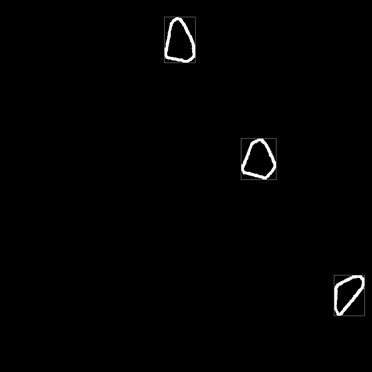

CPU times: user 63.6 ms, sys: 0 ns, total: 63.6 ms
Wall time: 39.3 ms

Everything put together has resulted in a detection algorithm that takes around 40 ms. This could be done in real time as it’s just about fast enough. A larger image would be slower though.

This was fun.