Binary Embeddings

There has been some recent interest in compressing embeddings. I was linked to the Matryoshka Representation Learning paper (Kusupati et al. 2024) through a chain of interesting blog posts. A huggingface blog post about embedding quantization lead to the MRL paper, and a post by Simon Willison about binary vector search suggests that the performance of binarized embeddings could be remarkably close to full precision.

Kusupati, Aditya, Gantavya Bhatt, Aniket Rege, Matthew Wallingford, Aditya Sinha, Vivek Ramanujan, William Howard-Snyder, et al. 2024. “Matryoshka Representation Learning.” https://arxiv.org/abs/2205.13147.

In this post I want to generate some embeddings, both from images and text, and explore how well a binarized version encodes them. First I will look at the approximate distribution of values and then I can measure how much the embedding compression reorders distance measurements betweeen embeddings.

Dataset

I already have imagenet downloaded so picking some images from that at random and embedding them with CLIP will provide a nice dataset to work with. For text there are several datasets I can use, and I can try out small and large models for embedding them.

from pathlib import Path
import pandas as pd

IMAGENET_FOLDER = Path("/data/image/imagenet/ILSVRC/Data/CLS-LOC/val") # this is a big dataset
IMAGENET_FILES = sorted(IMAGENET_FOLDER.glob("*.JPEG"))
IMAGENET_SELECTION = (
    pd.Series(IMAGENET_FILES)
        .sample(n=1_000, random_state=42)
        .tolist()
)

Code

from PIL import Image
from transformers import CLIPProcessor, CLIPVisionModel
from tqdm.auto import tqdm
import torch

class ClipEmbedder:
    def __init__(
        self,
        model_name: str = "openai/clip-vit-base-patch32",
        device: str | torch.device = "cuda",
    ) -> None:
        model = CLIPVisionModel.from_pretrained(model_name)
        self.model = model.to(device)
        self.processor = CLIPProcessor.from_pretrained(model_name)

    def embed(self, images: list[Path], batch_size: int = 8) -> torch.Tensor:
        return torch.concatenate(
            [
                self._embed(images[index:index+batch_size])
                for index in tqdm(range(0, len(images), batch_size))
            ]
        )

    @torch.inference_mode()
    def _embed(self, batch: list[Path]) -> torch.Tensor:
        images = map(Image.open, batch)
        images = [image.convert("RGB") for image in images]
        inputs = self.processor(
            images=images,
            return_tensors="pt",
            padding=True,
        )
        inputs = inputs.to(self.model.device)
        outputs = self.model(
            **inputs,
            output_attentions=False,
            output_hidden_states=False,
        )
        embeddings = outputs.pooler_output
        return embeddings.cpu()

image_embedder = ClipEmbedder()
image_embeddings = image_embedder.embed(IMAGENET_SELECTION)

image_embeddings.shape

torch.Size([1000, 768])

We have our embeddings and it was nice and quick to generate them. Let’s try for the text now.

I’m going to use the Sentiment 140 dataset (Go, Bhayani, and Huang 2009) which consists of sentiment bearing tweets. These are going to be short documents, depending on how this goes I might try with longer form documents.

Go, Alec, Richa Bhayani, and Lei Huang. 2009. “Twitter Sentiment Classification Using Distant Supervision.” CS224N Project Report, Stanford 1 (12): 2009.

import pandas as pd

text_df = pd.read_parquet("/data/sentiment/sentiment140/sentiment.gz.parquet")
TWEET_SELECTION = (
    text_df.sample(n=1_000, random_state=42)
        .text
        .tolist()
)

Code

from transformers import AutoTokenizer, AutoModel
from tqdm.auto import tqdm
import torch
import torch.nn.functional as F

class TextEmbedder:
    def __init__(
        self,
        model_name: str = "sentence-transformers/all-MiniLM-L6-v2",
        device: str | torch.device = "cuda",
    ) -> None:
        model = AutoModel.from_pretrained(model_name)
        self.model = model.to(device)
        self.tokenizer = AutoTokenizer.from_pretrained(model_name)

    def embed(self, documents: list[str], batch_size: int = 8) -> torch.Tensor:
        return torch.concatenate(
            [
                self._embed(documents[index:index+batch_size])
                for index in tqdm(range(0, len(documents), batch_size))
            ]
        )

    @torch.inference_mode()
    def _embed(self, batch: list[str]) -> torch.Tensor:
        inputs = self.tokenizer(
            batch,
            padding=True,
            truncation=True,
            return_tensors="pt",
        )
        inputs = inputs.to(self.model.device)
        outputs = self.model(
            **inputs,
            output_attentions=False,
            output_hidden_states=False,
        )
        embeddings = outputs.pooler_output
        return embeddings.cpu()

text_embedder = TextEmbedder()
text_embeddings = text_embedder.embed(TWEET_SELECTION)

loading configuration file config.json from cache at /home/matthew/.cache/huggingface/hub/models--sentence-transformers--all-MiniLM-L6-v2/snapshots/8b3219a92973c328a8e22fadcfa821b5dc75636a/config.json
Model config BertConfig {
  "_name_or_path": "sentence-transformers/all-MiniLM-L6-v2",
  "architectures": [
    "BertModel"
  ],
  "attention_probs_dropout_prob": 0.1,
  "classifier_dropout": null,
  "gradient_checkpointing": false,
  "hidden_act": "gelu",
  "hidden_dropout_prob": 0.1,
  "hidden_size": 384,
  "initializer_range": 0.02,
  "intermediate_size": 1536,
  "layer_norm_eps": 1e-12,
  "max_position_embeddings": 512,
  "model_type": "bert",
  "num_attention_heads": 12,
  "num_hidden_layers": 6,
  "pad_token_id": 0,
  "position_embedding_type": "absolute",
  "transformers_version": "4.37.2",
  "type_vocab_size": 2,
  "use_cache": true,
  "vocab_size": 30522
}

loading weights file model.safetensors from cache at /home/matthew/.cache/huggingface/hub/models--sentence-transformers--all-MiniLM-L6-v2/snapshots/8b3219a92973c328a8e22fadcfa821b5dc75636a/model.safetensors
All model checkpoint weights were used when initializing BertModel.

All the weights of BertModel were initialized from the model checkpoint at sentence-transformers/all-MiniLM-L6-v2.
If your task is similar to the task the model of the checkpoint was trained on, you can already use BertModel for predictions without further training.
loading file vocab.txt from cache at /home/matthew/.cache/huggingface/hub/models--sentence-transformers--all-MiniLM-L6-v2/snapshots/8b3219a92973c328a8e22fadcfa821b5dc75636a/vocab.txt
loading file tokenizer.json from cache at /home/matthew/.cache/huggingface/hub/models--sentence-transformers--all-MiniLM-L6-v2/snapshots/8b3219a92973c328a8e22fadcfa821b5dc75636a/tokenizer.json
loading file added_tokens.json from cache at None
loading file special_tokens_map.json from cache at /home/matthew/.cache/huggingface/hub/models--sentence-transformers--all-MiniLM-L6-v2/snapshots/8b3219a92973c328a8e22fadcfa821b5dc75636a/special_tokens_map.json
loading file tokenizer_config.json from cache at /home/matthew/.cache/huggingface/hub/models--sentence-transformers--all-MiniLM-L6-v2/snapshots/8b3219a92973c328a8e22fadcfa821b5dc75636a/tokenizer_config.json

text_embeddings.shape

torch.Size([1000, 384])

The text embeddings are much smaller as this is a much smaller model.

Embedding Distribution

When I was looking into the CLIP embedding generation I was surprised to find that most of the values were near zero. The blog post by Simon Willison also states the same thing. It would be good to check that this is generally true of the embeddings that I have generated.

Code

import pandas as pd

(
    pd.DataFrame(map(sorted, image_embeddings.tolist()))
        .sample(n=5, random_state=42)
        .T
        .plot(title="5 Image Embeddings", legend=False)
) ; None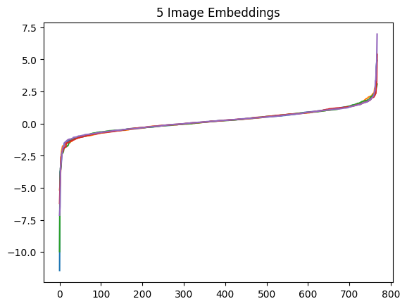

This is an extremely consistent distribution. We can check that this isn’t due to the sorting by viewing the unsorted embeddings.

Code

import pandas as pd

(
    pd.DataFrame(image_embeddings.tolist())
        .sample(n=5, random_state=42)
        .T
        .plot(title="5 Image Embeddings", legend=False)
) ; None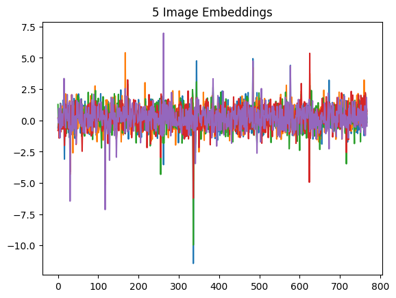

The embeddings do differ, however they have a consistent distribution of values across the embedding. I think that this will be a key aspect of the compression performance.

How do the text embeddings compare?

Code

import pandas as pd

(
    pd.DataFrame(map(sorted, text_embeddings.tolist()))
        .sample(n=5, random_state=42)
        .T
        .plot(title="5 Text Embeddings", legend=False)
) ; None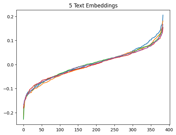

The text embeddings do have extremal values however they also have a smoother distribution of values. This should provide a good comparison for compression.

Ranking

With these I should be able to produce a distance matrix which is the distance between each pair of embeddings. Then after compressing these I can compare how the ranking of the distances has changed.

The aim of this is to measure the compressed embeddings in a way that is consistent with how I would use them. Embeddings for images or text are useful if they contain a semantic encoding of the source. Such embeddings can then be compared to each other to see if they represent similar concepts.

Compressing the embeddings is going to change the distance between two points. If it doesn’t change the ranking of the distances then it’s possible to produce the same clustering given a compressed embedding.

To ensure that my arbitrary metric is useful I am also going to measure the change using the Kendall rank correlation coefficient as well: > Intuitively, the Kendall correlation between two variables will be high when observations have a similar (or identical for a correlation of 1) rank (i.e. relative position label of the observations within the variable: 1st, 2nd, 3rd, etc.) between the two variables, and low when observations have a dissimilar (or fully different for a correlation of −1) rank between the two variables.

I can also normalize the embeddings and then compare distance changes using that. Ideally the normalization will account for the difference in dimensionality.

Code

import numpy as np
from scipy.stats import zscore
from scipy.stats import kendalltau

def reorder_score(original: np.array, comparison: np.array) -> float:
    original_argsort = original.argsort()
    comparison_argsort = comparison.argsort()
    matches = original_argsort == comparison_argsort
    return matches.mean()

def kendall_tau_score(original: np.array, comparison: np.array) -> float:
    original_argsort = original.argsort()
    comparison_argsort = comparison.argsort()
    value, pvalue = kendalltau(original_argsort, comparison_argsort)
    return value

def normalized_difference_score(original: np.array, comparison: np.array) -> float:
    original_normalized = zscore(original)
    comparison_normalized = zscore(comparison)
    difference = (original_normalized - comparison_normalized)
    abs_difference = np.abs(difference)
    return abs_difference.mean()

PCA Compression

One way to compress the embeddings is to reduce the dimensionality of the embeddings using PCA. This is a linear transform over the embedding space into a space with fewer dimensions which loses the least amount of information.

Code

from sklearn.metrics.pairwise import euclidean_distances
from tqdm.auto import tqdm
import numpy as np
from sklearn.decomposition import PCA

def full_pca_comparison(embeddings: np.array) -> pd.DataFrame:
    df = pd.DataFrame([
        pca_comparison(embeddings, dimensions=dimensions)
        for dimensions in tqdm(range(1, embeddings.shape[1]+1))
    ])
    return df

def pca_comparison(embeddings: np.array, dimensions: int) -> dict[str, float]:
    distances = euclidean_distances(embeddings)
    embeddings_pca = apply_pca(embeddings, dimensions=dimensions)
    distances_pca = euclidean_distances(embeddings_pca)

    reorder = reorder_score(distances, distances_pca)
    difference = normalized_difference_score(distances, distances_pca)
    kendall_tau = kendall_tau_score(distances, distances_pca)

    return {
        "reorder_score": reorder,
        "difference_score": difference,
        "kendall_tau_score": kendall_tau,
    }

def apply_pca(embeddings: np.array, dimensions: int, random_state: int = 0) -> np.array:
    pca = PCA(n_components=dimensions, random_state=random_state)
    pca_embeddings = pca.fit_transform(embeddings)
    return pca_embeddings

Code

from tqdm.auto import tqdm
import pandas as pd

image_pca_comparison_df = full_pca_comparison(image_embeddings)
image_pca_comparison_df.plot(title="Image Embedding PCA Compression") ; None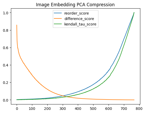

Code

from tqdm.auto import tqdm
import pandas as pd

text_pca_comparison_df = full_pca_comparison(text_embeddings)
text_pca_comparison_df.plot(title="Text Embedding PCA Compression") ; None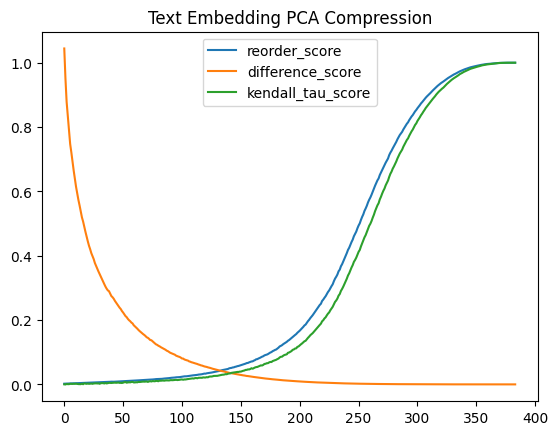

The difference score for these graphs grows as the normalized PCA distance differs from the original normalized distance. This means that as the value grows the distances between the PCA embeddings differs from the original more, so lower is better.

For the Kendall Tau and Reorder scores the comparison is between the original embeddings sorted by distance and the PCA embeddings. When the rankings are identical both of these scores are at their maximum value, so higher is better.

These graphs show me that the rankings are very quick to change while the actual distances are preserved quite well. The distances only really start to break down at around 20% of the original dimension count, while the rankings have significantly changed by that point.

Finally the image embeddings degrade faster than the text embeddings. I’m very surprised by this as the image embeddings are far more opinionated.

Binary Compression

In the Simon Willison blog post he talks about binarized embeddings, stating:

Binary vector search is a trick where you take that sequence of floating point numbers and turn it into a binary vector—just a list of 1s and 0s, where you store a 1 if the corresponding float was greater than 0 and a 0 otherwise.

I am not sure that this will work well with the embeddings that I have so far. Let’s see.

Code

from sklearn.metrics.pairwise import euclidean_distances

def binary_comparison(embeddings: np.array) -> dict[str, float]:
    distances = euclidean_distances(embeddings)
    embeddings_binary = embeddings > 0
    distances_binary = euclidean_distances(embeddings_binary)

    reorder = reorder_score(distances, distances_binary)
    difference = normalized_difference_score(distances, distances_binary)
    kendall_tau = kendall_tau_score(distances, distances_binary)

    return {
        "reorder_score": reorder,
        "difference_score": difference,
        "kendall_tau_score": kendall_tau,
    }

Code

pd.DataFrame([
    binary_comparison(image_embeddings),
    binary_comparison(text_embeddings),
], index=["image", "text"])

	reorder_score	difference_score	kendall_tau_score
image	0.006330	0.415055	0.003785
text	0.005015	0.454922	0.002242

This is terrible.

Code

print("Image PCA Compression, 35-45 dimensions")
image_pca_comparison_df.iloc[35:45]

Image PCA Compression, 35-45 dimensions

	reorder_score	difference_score	kendall_tau_score
35	0.005844	0.451231	0.004154
36	0.005891	0.446154	0.002432
37	0.006025	0.444435	0.003185
38	0.005982	0.440945	0.003320
39	0.006031	0.436580	0.002555
40	0.006125	0.433233	0.003144
41	0.006046	0.432521	0.002665
42	0.006145	0.428558	0.003102
43	0.006229	0.424315	0.003757
44	0.006309	0.420885	0.003475

Code

print("Text PCA Compression, 15-25 dimensions")
text_pca_comparison_df.iloc[15:25]

Text PCA Compression, 15-25 dimensions

	reorder_score	difference_score	kendall_tau_score
15	0.004360	0.519220	0.002216
16	0.004487	0.506223	0.000527
17	0.004657	0.489764	0.003345
18	0.004721	0.474116	0.002310
19	0.005042	0.459233	0.001773
20	0.005079	0.444529	0.002508
21	0.005278	0.431021	0.001737
22	0.005468	0.420118	0.002280
23	0.005463	0.407732	0.002590
24	0.005699	0.398507	0.001784

These results suggest to me that the binary embeddings are around 20 (text) or 40 (image) dimensions. Remember that the image embeddings are twice as big as the text ones.

Overall this is far less impressive than I expected given the recent hype around all this.